Sample Variance
Population mean is a parameter. Sample mean is a statistic, to estimate that parameter.
Population variance is also a parameter that we may like to estimate. We can follow the same steps as we take while calculating the population variance, but this time with the sample mean.

The result would be a close estimate but not the best estimate that we can make, given the data we have. Because it would underestimate it. Below, we’ll look at it closely but it turns out, we’re going to get a better estimate for our population variance if we don’t divide by the number of data points we have but we divide by one less than the number of data points we have.
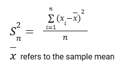
So the standard definition of sample variance is:

Why do we divide by n – 1 in variance?
Now let’s check why we are dividing by n-1. Below are three videos about this matter.
Intro: A Quick Demonstration
First, let’s have a quick view at the effects of diving by different values.
Here is the video by Khan Academy that demonstrates what happens when we divide by n, n-1 and n-2.
And here is the link to that code used in the video, prepared by Justin Helps.
Showing Bias in Sample Variance
For a deeper look, now we can check the video below that shows bias in sample variance (when we divide by n).
This demonstration shows us:
By checking the Sample mean vs. Biased Sample variance chart:
- The cases where we are significantly underestimating the sample variance, we are getting sample variances close to zero and these are also (disproportionately) the cases where the means for those samples are way far off from the true mean.
- On those tails (the above cases) we mostly have smaller sample sizes. (red ones are smaller size than the blue ones)
By checking the Sample size vs. Biased Sample var./Population var. (%) chart:
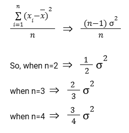
- If we keep taking sample size ‘2’ over many trials and keep calculating the biased sample variances and dividing that by the population variance, it’s approaching half of the true population variance.
- When the sample size is ‘3’, it’s approaching 2/3 of the true population variance.
- When the sample size is ‘4’, it’s approaching 3/4 of the true population variance.
We can come up with the general theme here:
When we use the biased estimate, we’re not approaching the population variance. Instead, we are approaching n-1 over n times the population variance.

This is giving us a biased estimate. To unbias this (to get our best estimate of the true population variance), we’d want to multiple n over n-1.

Here is the link to that code used in the video, prepared by Peter Collingridge.
Simulation providing evidence that (n-1) gives us unbiased estimate
Let’s check a simulation that shows how to get an unbiased estimate.
This above video by Khan Academy simulates the graphs showing results of the following formula, where a differs from -3 till 1. So we’ll be able to see the changes within that range.
Variance = Sum ((x[i]-mean(x))²) / (n+a)
With this code we can simulate many samples and it gives us a curve. When we average together those curves from all the samples it created, we see our best estimate is when a is pretty close to negative 1.
Anything less than negative 1, we start overestimating the variance.
And here is the link to that code used in the video, prepared by Tetef.
Sample standard deviation and bias
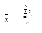
The formal way to write the formula of sample mean is:

This would be our estimate of what the population mean might be. But we would like to check the spread as well to understand how much our measurements vary from the sample mean.
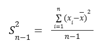
So the formula of the unbiased sample variance is:

That is an unbiased estimate of population variance (when we divide by n – 1). To get the sample standard deviation, we just take the square root of the unbiased sample variance.

However, because the square root function is nonlinear, it turns out this above is not an unbiased estimate of true population standard deviation.
Remember, to unbias the sample variance, we just had to divide by n-1, instead of n and that would work for any probability distribution. BUT it turns out, to do the same thing for standard deviation, it’s not that easy. It’s actually dependent on how that population is actually distributed.
It’s biased but it’s the simplest, best tool we have.
Box Plots and Outliers
Box and whisker plots seek to explain data by showing a spread of all the data points in a sample. A box and whisker plot—also called a box plot—displays the five-number summary of a set of data. The five-number summary is the minimum, first quartile, median, third quartile, and maximum.
The box part essentially represents the middle half of our data. Another way to tell is, the data between the medians of the two halves. And the whiskers part essentially shows the range of our data. They are two opposite ends of the data.
The five-number summary divides the data into sections that each contain approximately 25% of the data in that set. (Median is the Q2.)
Outliers
An outlier is a data point that lies outside the overall pattern in a distribution.
Statisticians have developed many ways to identify what should and shouldn’t be called an outlier. A commonly used rule says that a data point is an outlier if it is more than 1.5 IQR above the third quartile or below the first quartile.
low outliers = Q1-1.5 IQR
high outliers = Q3+1.5 IQR
Box and whisker plots will often show outliers as dots that are separate from the rest of the plot.
Other Measures of Spread
Range and mid-range
The range is the difference between the largest and smallest data points in a set of numerical data. The midrange is the average of the largest and smallest data points. Range is an easy to calculate measure of variability, while midrange is an easy to calculate measure of central tendency.
Mean absolute deviation
Mean absolute deviation (MAD) of a data set is the average distance between each data value and the mean. Mean absolute deviation is a way to describe variation in a data set. Mean absolute deviation helps us get a sense of how “spread out” the values in a data set are.

Standard Deviation or Mean Absolute Deviation ?
Standard deviation is more complicated, but it has some nice properties that make it a preferred measure of spread for statisticians.
Disclaimer: Like most of my posts, this content is intended solely for educational purposes and was created primarily for my personal reference. At times, I may rephrase original texts, and in some cases, I include materials such as graphs, equations, and datasets directly from their original sources.
I typically reference a variety of sources and update my posts whenever new or related information becomes available. For this particular post, the primary source was Khan Academy’s Statistics and Probability series.
