Like we did before when we run a simple linear regression, we’ll assume that we are part of an analytics team that provides insights about marketing and sales. We have been assigned to a project that focuses on the use of influencer marketing, and we would like to explore the relationship between marketing promotional budgets and sales.
The dataset provided includes information about marketing campaigns across TV, radio, and social media, as well as how much revenue in sales was generated from these campaigns. Based on this information, leaders in our company will make decisions about where to focus future marketing efforts, so it is critical to have a clear understanding of the relationship between the different types of marketing and the revenue they generate.
Imports & Load the dataset
# Import pandas, pyplot from matplotlib, and seaborn.
import pandas as pd
import matplotlib.pyplot as plt
import seaborn as sns

# Import the statsmodel module.
import statsmodels.api as sm

# Import the ols function from statsmodels.
from statsmodels.formula.api import ols
This is a fictional dataset that was created for educational purposes. The variables in the dataset have been kept as is to suit the objectives of this activity.
# Load the data.
data = pd.read_csv('marketing_and_sales_data_evaluate_lr.csv')

# Display the first five rows.
data.head()| TV | Radio | Social_Media | Sales | |
|---|---|---|---|---|
| 0 | 16.0 | 6.566231 | 2.907983 | 54.732757 |
| 1 | 13.0 | 9.237765 | 2.409567 | 46.677897 |
| 2 | 41.0 | 15.886446 | 2.913410 | 150.177829 |
| 3 | 83.0 | 30.020028 | 6.922304 | 298.246340 |
| 4 | 15.0 | 8.437408 | 1.405998 | 56.594181 |
Data exploration
The features in the data are:
- TV promotion budget (in millions of dollars)
- Social media promotion budget (in millions of dollars)
- Radio promotion budget (in millions of dollars)
- Sales (in millions of dollars)
Each row corresponds to an independent marketing promotion where the business invests in TV, Social_Media, and Radio promotions to increase Sales.
The business would like to determine which feature most strongly predicts Sales so they have a better understanding of what promotions they should invest in in the future. To accomplish this, we’ll construct a simple linear regression model that predicts sales using a single independent variable.
# Display the shape of the data as a tuple (rows, columns)
data.shape
(4572, 4)
Explore the independent variables
# Generate descriptive statistics about TV, Radio, and Social_Media.
data[['TV','Radio','Social_Media']].describe()| TV | Radio | Social_Media | |
|---|---|---|---|
| count | 4562.000000 | 4568.000000 | 4566.000000 |
| mean | 54.066857 | 18.160356 | 3.323956 |
| std | 26.125054 | 9.676958 | 2.212670 |
| min | 10.000000 | 0.000684 | 0.000031 |
| 25% | 32.000000 | 10.525957 | 1.527849 |
| 50% | 53.000000 | 17.859513 | 3.055565 |
| 75% | 77.000000 | 25.649730 | 4.807558 |
| max | 100.000000 | 48.871161 | 13.981662 |
Explore the dependent variable
Before fitting the model, ensure the Sales for each promotion (i.e., row) is present. If the Sales in a row is missing, that row isn’t of much value to the simple linear regression model.
Display the percentage of missing values in the Sales column in the DataFrame data.
# Calculate the average missing rate in the sales column.
missing_sales = data.Sales.isna().mean()

# Convert the missing_sales from a decimal to a percentage and round to 2 decimal places.
missing_sales = round(missing_sales*100, 2)

# Display the results (missing_sales must be converted to a string to be concatenated in the print statement).
print('Percentage of promotions missing Sales: ' +  str(missing_sales) + '%')
Percentage of promotions missing Sales: 0.13%
- 0.13% of rows are missing the
Salesvalue.
Remove the missing data
# Subset the data to include rows where Sales is present.
data = data.dropna(subset = ['Sales'], axis = 0)
Visualize the sales distribution
# Create a histogram of the Sales.
fig = sns.histplot(data['Sales'])
# Add a title
fig.set_title('Distribution of Sales');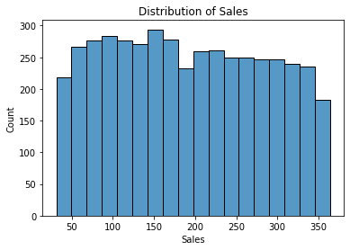
- Generally,
Salesare equally distributed between 25 and 350 million.
Model building
We will use a pairplot to visually determine which variable has the strongest linear relationship with Sales. This will help us select the X variable for the simple linear regression.
# Create a pairplot of the data.
sns.pairplot(data)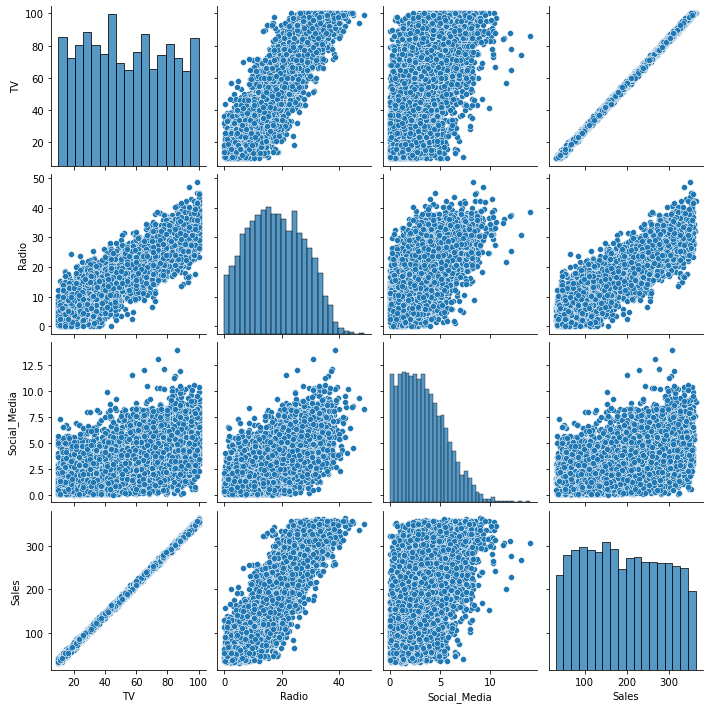
TVclearly has the strongest linear relationship withSales.RadioandSalesappear to have a linear relationship, but there is larger variance than betweenTVandSales.
Build and fit the model
# Define the OLS formula.
ols_formula = 'Sales ~ TV'

# Create an OLS model.
OLS = ols(formula = ols_formula, data = data)

# Fit the model.
model = OLS.fit()

# Save the results summary.
model_results = model.summary()

# Display the model results.
model_results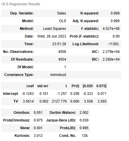
Warnings:
[1] Standard Errors assume that the covariance matrix of the errors is correctly specified.
Check model assumptions
To justify using simple linear regression, check that the four linear regression assumptions are not violated. These assumptions are:
- Linearity
- Independent Observations
- Normality
- Homoscedasticity
Model assumption: Linearity
The linearity assumption requires a linear relationship between the independent and dependent variables.
# Create a scatterplot comparing X and Sales (Y).
sns.scatterplot(x = data['TV'], y = data['Sales'])
- There is a clear linear relationship between
TVandSales, meeting the linearity assumption.
Model assumption: Independence
The independent observation assumption states that each observation in the dataset is independent. As each marketing promotion (i.e., row) is independent from one another, the independence assumption is not violated.
Model assumption: Normality
The normality assumption states that the errors are normally distributed.
We’ll create two plots to check this assumption:
- Plot 1: Histogram of the residuals
- Plot 2: Q-Q plot of the residuals
# Calculate the residuals
residuals = model.resid

# Create a 1x2 plot figure
fig, axes = plt.subplots(1, 2, figsize = (8,4))

# Create a histogram with the residuals
sns.histplot(residuals, ax=axes[0])
# Set the x label of the residual plot
axes[0].set_xlabel("Residual Value")
# Set the title of the residual plot
axes[0].set_title("Histogram of Residuals")

# Create a Q-Q plot of the residuals
sm.qqplot(residuals, line='s',ax = axes[1])
# Set the title of the Q-Q plot
axes[1].set_title("Normal Q-Q plot")

# Use matplotlib's tight_layout() function to add space between plots for a cleaner appearance
plt.tight_layout()
# Show the plot.
plt.show()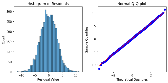
- The histogram of the residuals are approximately normally distributed, which supports that the normality assumption is met for this model. The residuals in the Q-Q plot form a straight line, further supporting that the normality assumption is met.
Model assumption: Homoscedasticity
The homoscedasticity (constant variance) assumption is that the residuals have a constant variance for all values of X.
# Create a scatterplot with the fitted values from the model and the residuals
fig = sns.scatterplot(x = model.fittedvalues, y = model.resid)

# Set the x-axis label
fig.set_xlabel("Fitted Values")
# Set the y-axis label
fig.set_ylabel("Residuals")
# Set the title
fig.set_title("Fitted Values v. Residuals")

# Add a line at y = 0 to visualize the variance of residuals above and below 0
fig.axhline(0)
# Show the plot.
plt.show()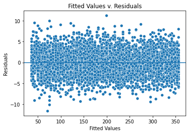
- The variance of the residuals is consistent across all X. Thus, the assumption of homoscedasticity is met.
Results and evaluation
Display the OLS regression results
If the linearity assumptions are met, we can interpret the model results accurately.
# Display the model_results defined previously
model_results
Warnings:
[1] Standard Errors assume that the covariance matrix of the errors is correctly specified.
- Using
TVas X results in a simple linear regression model with R2=0.999. In other words,TVexplains 99.9% of the variation inSales.
The R-squared value will depend on the variable selected for X.
Interpret the model results
With the model fit evaluated, we can assess the coefficient estimates and the uncertainty of these estimates.
- When
TVis used as the independent variable X, the coefficient for theInterceptis -0.1263 and the coefficient forTVis 3.5614.
- When
TVis used as the independent variable X, the linear equation is:
Y = Intercept + Slope ∗ X
Sales (in millions) = Intercept + Slope ∗ TV (in millions)
Sales (in millions) = −0.1263 + 3.5614 ∗ TV (in millions)
- According to the model, when
TVis used as the independent variable X, an increase of one million dollars for the TV promotional budget results in an estimated 3.5614 million dollars more in sales.
- Beta coefficients allow us to estimate the magnitude and direction (positive or negative) of the effect of each independent variable on the dependent variable. The coefficient estimates can be converted to explainable insights, such as the connection between an increase in TV promotional budgets and sales.
Measure the uncertainty of the coefficient estimates
Model coefficients are estimated. This means there is an amount of uncertainty in the estimate. A p-value and 95% confidence interval are provided with each coefficient to quantify the uncertainty for that coefficient estimate.
- When
TVis used as the independent variable, it has a p-value of 0.0000.000 and a 95% confidence interval of [3.558,3.565][3.558,3.565]. This means there is a 95% chance the interval [3.558,3.565][3.558,3.565] contains the true parameter value of the slope. These results indicate little uncertainty in the estimation of the slope of X. Therefore, the business can be confident in the impactTVhas onSales.
- Potential areas to explore include:
- Providing the business with the estimated sales given different TV promotional budgets
- Using both
TVandRadioas independent variables - Adding plots to help convey the results, such as using the
seabornregplot()to plot the data with a best fit regression line
- Of the three available promotion types (TV, radio, and social media), TV has the strongest positive linear relationship with sales. According to the model, an increase of one million dollars for the TV promotional budget will result in an estimated 3.5614 million dollars more in sales. This is a very confident estimate, as the p-value for this coefficient estimate is small. Thus, the business should prioritize increasing the TV promotional budget over the radio and social media promotional budgets to increase sales.
Considerations
What are some key takeaways?
- Exploratory data analysis can be used to find a suitable X variable for a simple linear regression model.
- It’s important to check that simple linear regression assumptions are met before interpreting model results.
- R-squared is a useful measure of prediction error.
- It’s important to provide measures of uncertainty (e.g., p-values, confidence intervals) with any coefficient estimates.
What findings could we share with others?
- Sales is relatively equally distributed between $25 and $350 million across all promotions.
- In the data visualization, TV has the strongest linear relationship with sales. Radio and sales appear to have a moderate linear relationship, but there is larger variance than between TV and sales. Social media and sales appear to have a weak linear relationship.
- When TV is used as the independent variable, the R-squared for the simple linear regression model estimating sales is 0.999.
- When TV is used as the independent variable, the coefficient for the intercept is -0.1263 and the coefficient for TV is 3.5614.
- When TV is used as the independent variable, the slope of the coefficient for TV has a p-value of 0.000 and a 95% confidence interval of [3.558, 3.565].
How could we frame your findings to stakeholders?
- Among TV, social media, and radio, TV had the strongest positive linear relationship with sales.
- The linear regression model estimates that 99.9% of the variation in sales is explained by the TV promotional budget. In other words, nearly all of the variation in sales can be explained by the TV promotional budget alone, making TV an excellent predictor of sales.
- According to the model, when TV is used as the independent variable X, an increase of one million dollars for the TV promotional budget would result in an estimated 3.5614 million more dollars in sales.
- The interval (3.558 million, 3.565 million) has a 95% probability of containing the true estimate of the increase in sales for a one million dollar increase in the TV promotional budget. Therefore, the estimate provided in the previous bullet is very confident.
Disclaimer: Like most of my posts, this content is intended solely for educational purposes and was created primarily for my personal reference. At times, I may rephrase original texts, and in some cases, I include materials such as graphs, equations, and datasets directly from their original sources.
I typically reference a variety of sources and update my posts whenever new or related information becomes available. For this particular post, the primary source was Google Advanced Data Analytics Professional Certificate.