We’ll focus more on categorical variables now. We can start asking questions like:
- Is the difference among three or more groups statistically significant?
- Is the distribution of observed data different from what we expected?
Hypothesis testing is a statistical procedure that uses sample data to evaluate an assumption about a population parameter.
Chi-squared test (x2) will help us determine if two categorical variables are associated with one another, and whether a categorical variable follows unexpected distribution.
Hypothesis testing with chi-squared
Chi-squared tests are used to determine whether one or more observed categorical variables follow expected distribution(s). Here we’ll check two main chi-squared tests; goodness of fit and test for independence, which can be used to test our expected hypothesis against what actually occurred.
The Chi-squared goodness of fit test
The chi-squared (X2) goodness of fit test determines whether an observed categorical variable (with more than two possible levels) follows an expected distribution.
Null Hypothesis (H0)
- The variable follows the expected distribution
Alternative Hypothesis (H1)
- The variable does NOT follow the expected distribution
Let’s consider the scenario below that will define the null and alternative hypotheses (based on the scenario), set up a Goodness of Fit test, evaluate the test results, and draw a conclusion.
Chi-squared goodness of fit scenario
Imagine that for an online clothing company, that they expect the number of website visitors to be the same for each day of the week. We decide to test their hypothesis and pull data every day for the next week and record the number of website visitors in the table below.
| Day of the Week | Observed Values |
| Sunday | 650 |
| Monday | 570 |
| Tuesday | 420 |
| Wednesday | 480 |
| Thursday | 510 |
| Friday | 380 |
| Saturday | 490 |
| Total | 3,500 |
Here are the main steps we will take:
- Identify the Null and Alternative Hypotheses
- Calculate the chi-square test statistic (X2)
- Calculate the p-value
- Make a conclusion
Step 1: Identify the null and alternative hypotheses
H0: The week we observed follows their expectations that the number of website visitors is equal on any given day.
Ha: The week we observed does not follow their expectations; therefore, the number of website visitors is not equal across the days of the week.
Step 2: Calculate the chi-squared test statistic (X2)
We need to calculate a test statistic to determine if we should reject or fail to reject our null hypothesis. This test statistic is known as the chi-squared statistic and is calculated based on the following formula:
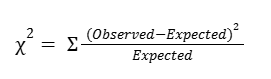
The intuition behind this formula is that it should quantify the extent of any discrepancies between observed frequencies and expected frequencies for each categorical level. Squaring these differences does two things:
- First, it ensures that all discrepancies between observed and expected contribute positively to the chi-squared statistic.
- Second, it penalizes larger discrepancies.
Dividing the sum of the squared differences by the expected frequency of each category level standardizes the differences. In other words, it accounts for the fact that larger discrepancies are more significant when the expected frequencies are small, and less so when the expected frequencies are large.
Returning to the example, since there were a total of 3,500 website visitors we observed; their expectation is that 500 visitors would visit each day (3,500/7).
| Day of the Week | Observed Values | Chi-Squared Test Statistic |
| Sunday | 650 | (650-500)2 / 500 = 45 |
| Monday | 570 | (570-500)2 / 500 = 9.8 |
| Tuesday | 420 | (420-500)2 / 500 = 12.8 |
| Wednesday | 480 | (480-500)2 / 500 = 0.8 |
| Thursday | 510 | (510-500)2 / 500 = 0.2 |
| Friday | 380 | (380-500)2 / 500 = 28.8 |
| Saturday | 490 | (490-500)2 / 500 = 0.2 |
The 𝛸2 statistic would be the sum of the third column above:
𝛸2 = 45 + 9.8 + 12.8 + 0.8 + 0.2 + 28.8 + 0.2 = 97.6
Note that the 𝛸2 goodness of fit test does not produce reliable results when there are any expected values of less than five.
Step 3: Find the p-value
What is the probability of obtaining a 𝛸2 statistic of 97.6 or greater when examining 3,500 website visits if the null hypothesis is true? This is the question that the p-value or “observed significance level” will answer.
A long time ago, Pearson realized that p-values for 𝛸2 statistics very closely corresponded with areas under certain curves, known as 𝛸2 curves. 𝛸2 curves represent probability density functions, and their shapes vary based on how many degrees of freedom are present in the experiment.
Degrees of Freedom
Degrees of freedom are determined by the model, not by the data. This means that, in the website traffic example, the degrees of freedom are determined by how many different days a given visit can occur on, not by how many visits are sampled nor by the daily frequencies of the samples themselves. When the model is fully specified (i.e., we know all the possible categorical levels), then:
degrees of freedom = number of categorical levels – 1
In our example, there are seven categorical levels (one for each day of the week). Therefore, there are six degrees of freedom. This is because the counts of each level (day) are free to fluctuate, but once we know the counts for six days, the seventh day cannot vary. It must result in a total of 3,500 when summed with the other six days.
The following figure depicts the 𝛸2 curves for three different degrees of freedom: five, 10, and 20.

The p-value for a given 𝛸2 test statistic is very closely approximated by the area to its right beneath the 𝛸2 curve of the appropriate degrees of freedom. Notice that the more degrees of freedom there are in the experiment, the greater the area under the right tail of the curve for any given 𝛸2 test statistic, and therefore the greater the probability of getting a given 𝛸2 test statistic if the null hypothesis is true.
The following figure contains the 𝛸2 curve for six degrees of freedom. For a 𝛸2 test statistic of, for instance, 10, the value of P is approximated by the shaded area under the curve where x ≥ 10.

In the case of the website visits, there are six degrees of freedom, but the 𝛸2 test statistic is 97.6, that is far along the x-axis in the right-skewed tail of the curve. The area under this interval is miniscule: 7.94e-17.
In other words, the chances of getting a 𝛸2 test statistic ≥ 97.6 from 3,500 website visits if the null hypothesis were true are 7.94e-17%; practically zero.
Step 4: Make a conclusion
Since the p-value is far less than 0.05, there is sufficient evidence to suggest that the number of visitors is not equal per day.
Coding
Thankfully, we don’t need to manually calculate our 𝛸2 test statistic or determine P by hand. We can use the chisquare() function from Python’s scipy.stats package to do this. The following code uses our observed and expected values to calculate the chi-squared test statistic and the p-value.
Note that the degrees of freedom are set to the number of observed frequencies minus one. This can be adjusted using the ddof parameter, but note that this parameter represents k – 1 – ddof degrees of freedom, where k is the number of observed frequencies. So, by default, ddof=0 when we call the function, and setting ddof=1 means that our degrees of freedom are reduced by two.
import scipy.stats as stats
observations = [650, 570, 420, 480, 510, 380, 490]
expectations = [500, 500, 500, 500, 500, 500, 500]
result = stats.chisquare(f_obs=observations, f_exp=expectations)
result
Power_divergenceResult(statistic=97.599999999999994, pvalue=7.9438869233438347e-19)
The output confirms our calculation of the chi-square test statistic in Step 2 and also gives us the associated p-value. Because the p-value is less than the significance level of 5%, we can reject the null hypothesis.
The chi-squared test for independence
The chi-squared (X2) test for independence (also called a test of homogeneity) determines whether or not two categorical variables are associated with each other. It is valid when our data comes from a random sample and we want to make an inference about the general population.
Null Hypothesis (H0)
- Two categorical variables are independent
Alternative Hypothesis (Ha)
- Two categorical variables are not independent
Chi-squared test for independence scenario
Now suppose that we have been asked to expand our analysis to look at the relationship between the device that a website user used and their membership status.
In this example, the 𝛸2 test of independence determines whether the type of device a visitor uses to visit the website (Mac or PC) is dependent on whether they have a membership account or browses as a guest (member or guest).
Step 1: Identify the null and alternative hypotheses
H0: The type of device a website visitor uses to visit the website is independent of the visitor’s membership status.
Ha: The type of device a website visitor uses to visit the website is not independent of the visitor’s membership status.
Step 2: Calculate the chi-squared test statistic (𝛸2)
To calculate the 𝛸2 test statistic, we need to arrange the data as a table that contains m x n values, where m and n are the number of possible levels contained within each respective categorical variable.
| Observed Values | Member | Guest | Total |
| Mac | 850 | 450 | 1,300 |
| PC | 1,300 | 900 | 2,200 |
| Total | 2,150 | 1,350 | 3,500 |
To calculate the expected values, the formula is:
Expected values = (Column total * Row total) / Overall total
Or we can write as below.
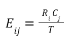
This can be read as: The expected value for the cell in the ith row and jth column is equal to the total of row_i times the total of column_j divided by the total count in the two-by-two table.
The formula comes from the definition of independence:
P(A and B) = P(A) * P(B)
For example, the expected value for a Mac member would be:
expected value = 2150 * 1300 / 3500 = 799
The logic of this calculation is as follows:
If device and membership status are truly independent, then the rate of Mac users who are members should be the same as the rate of Mac users who are guests.
The percentage of users who use Macs out of all the users is;
1,300 / 3,500 = 0.371 * 100 = 37.1%.
Accordingly, 37.1% of members and 37.1% of guests would be expected to use Macs.
So, 0.371 * 2,150 members ≈ 799.
The following table contains all the expected values:
| Expected Values | Member | Guest |
| Mac | 799 | 501 |
| PC | 1,351 | 849 |
Step 3: Find the p-value
Finding the p-value associated with a particular 𝛸2 test statistic is similar to the process outlined already for the goodness of fit test. The only minor difference is how to determine the number of degrees of freedom.
For an independence test with two categorical variables with m x n possible levels, there are (m – 1) (n – 1) degrees of freedom, assuming there are no other constraints on the probabilities. So, in the working example, this means there is (2 – 1)(2 – 1) = 1 degree of freedom. The p-value in this example is 0.00022. (It was determined using Python.)
Step 4: Make a conclusion
Because the p-value is 0.00022, we can reject the null hypothesis in favor of the alternative. We conclude that the type of device a website-user uses is not independent of his or her membership status.
We may recommend to our boss to dive into the reasons behind why visitors sign up for paid memberships more on a particular device. Perhaps the sign-up button appears differently on a particular device. Or maybe there are device-specific bugs that need to be fixed. These are just a couple examples of things we might consider for further exploration.
Coding
We can use the scipy.stats package’s chi2_contingency() function to obtain the 𝛸2 test statistic and p-value of a 𝛸2 independence test. The chi2_contingency() function only needs the observed values; it will calculate the expected values.
import numpy as np
import scipy.stats as stats
observations = np.array([[850, 450],[1300, 900]])
result = stats.contingency.chi2_contingency(observations, correction=False)
result
(13.660757846804358, 0.00021898310129108426, 1, array([[ 798.57142857, 501.42857143],[ 1351.42857143, 848.57142857]]))
The output above is in the following order: the 𝛸2 statistic, p-value, degrees of freedom, and expected values in array format.
One thing to note is that when degrees of freedom = 1 (i.e., we have a 2 x 2 table), the default behavior of the stats.chi2_contingency() function is to apply Yates’ correction for continuity. This is to make it less likely that small discrepancies will result in significant 𝛸2 values.
It is designed to be used when it’s possible for an expected frequency in the table to be small (generally < 5). In the given example, it is known that the expected values are all well over five. Therefore, the correction parameter was set to False.
Key takeaways
- The 𝛸2 goodness of fit test is used to test if an observed categorical variable follows a particular expected distribution.
- The 𝛸2 test for independence is used to test if two categorical variables are independent of each other or not (when samples are drawn at random and we want to make an inference about the whole population).
- Both 𝛸2 tests follow the same hypothesis testing steps to determine whether we should reject or fail to reject the null hypothesis to drive decision making.
Disclaimer: Like most of my posts, this content is intended solely for educational purposes and was created primarily for my personal reference. At times, I may rephrase original texts, and in some cases, I include materials such as graphs, equations, and datasets directly from their original sources.
I typically reference a variety of sources and update my posts whenever new or related information becomes available. For this particular post, the primary source was Google Advanced Data Analytics Professional Certificate.