Introduction
This activity is a continuation of the airlines project in which we built decision tree and random forest models. We will use the same data, but this time we will train, tune, and evaluate an XGBoost model. We’ll then compare the performance of all three models and decide which model is best. Finally, we’ll explore the feature importance of our model and identify the features that most contribute to customer satisfaction.
Step 1: Imports
# Import relevant libraries and modules
import numpy as np
import pandas as pd
import matplotlib as plt
import pickle

from sklearn.model_selection import train_test_split
from sklearn.model_selection import GridSearchCV
from sklearn import metrics

from xgboost import XGBClassifier
from xgboost import plot_importance
airline_data = pd.read_csv('Invistico_Airline.csv', error_bad_lines=False)# Display first ten rows of data
airline_data.head(10)| satisfaction | Customer Type | Age | Type of Travel | Class | Flight Distance | Seat comfort | Departure/Arrival time convenient | Food and drink | Gate location | … | Online support | Ease of Online booking | On-board service | Leg room service | Baggage handling | Checkin service | Cleanliness | Online boarding | Departure Delay in Minutes | Arrival Delay in Minutes | |
|---|---|---|---|---|---|---|---|---|---|---|---|---|---|---|---|---|---|---|---|---|---|
| 0 | satisfied | Loyal Customer | 65 | Personal Travel | Eco | 265 | 0 | 0 | 0 | 2 | … | 2 | 3 | 3 | 0 | 3 | 5 | 3 | 2 | 0 | 0.0 |
| 1 | satisfied | Loyal Customer | 47 | Personal Travel | Business | 2464 | 0 | 0 | 0 | 3 | … | 2 | 3 | 4 | 4 | 4 | 2 | 3 | 2 | 310 | 305.0 |
| 2 | satisfied | Loyal Customer | 15 | Personal Travel | Eco | 2138 | 0 | 0 | 0 | 3 | … | 2 | 2 | 3 | 3 | 4 | 4 | 4 | 2 | 0 | 0.0 |
| 3 | satisfied | Loyal Customer | 60 | Personal Travel | Eco | 623 | 0 | 0 | 0 | 3 | … | 3 | 1 | 1 | 0 | 1 | 4 | 1 | 3 | 0 | 0.0 |
| 4 | satisfied | Loyal Customer | 70 | Personal Travel | Eco | 354 | 0 | 0 | 0 | 3 | … | 4 | 2 | 2 | 0 | 2 | 4 | 2 | 5 | 0 | 0.0 |
| 5 | satisfied | Loyal Customer | 30 | Personal Travel | Eco | 1894 | 0 | 0 | 0 | 3 | … | 2 | 2 | 5 | 4 | 5 | 5 | 4 | 2 | 0 | 0.0 |
| 6 | satisfied | Loyal Customer | 66 | Personal Travel | Eco | 227 | 0 | 0 | 0 | 3 | … | 5 | 5 | 5 | 0 | 5 | 5 | 5 | 3 | 17 | 15.0 |
| 7 | satisfied | Loyal Customer | 10 | Personal Travel | Eco | 1812 | 0 | 0 | 0 | 3 | … | 2 | 2 | 3 | 3 | 4 | 5 | 4 | 2 | 0 | 0.0 |
| 8 | satisfied | Loyal Customer | 56 | Personal Travel | Business | 73 | 0 | 0 | 0 | 3 | … | 5 | 4 | 4 | 0 | 1 | 5 | 4 | 4 | 0 | 0.0 |
| 9 | satisfied | Loyal Customer | 22 | Personal Travel | Eco | 1556 | 0 | 0 | 0 | 3 | … | 2 | 2 | 2 | 4 | 5 | 3 | 4 | 2 | 30 | 26.0 |
10 rows × 22 columns
# Display the data type for each column in your DataFrame
airline_data.dtypes
satisfaction object Customer Type object Age int64 Type of Travel object Class object Flight Distance int64 Seat comfort int64 Departure/Arrival time convenient int64 Food and drink int64 Gate location int64 Inflight wifi service int64 Inflight entertainment int64 Online support int64 Ease of Online booking int64 On-board service int64 Leg room service int64 Baggage handling int64 Checkin service int64 Cleanliness int64 Online boarding int64 Departure Delay in Minutes int64 Arrival Delay in Minutes float64 dtype: object
Step 2: Model preparation
# Convert the object predictor variables to numerical dummies
airline_data_dummies = pd.get_dummies(airline_data,
                                         columns=['satisfaction','Customer Type','Type of Travel','Class'])
# Define the y (target) variable
y = airline_data_dummies['satisfaction_satisfied']
# Define the X (predictor) variables
= airline_data_dummies.drop(['satisfaction_satisfied','satisfaction_dissatisfied'], axis = 1)# Perform the split operation on data
X_train, X_test, y_train, y_test = train_test_split(X, y, test_size = 0.25, random_state = 0)Step 3: Model building
# Define xgb to be XGBClassifier
xgb = XGBClassifier(objective='binary:logistic', random_state=0)
Define the parameters for hyperparameter tuning
To identify suitable parameters for your xgboost model, first we need to define the parameters for hyperparameter tuning. Specifically, we’ll consider tuning max_depth, min_child_weight, learning_rate, n_estimators, subsample, and/or colsample_bytree.
Consider a more limited range for each hyperparameter to allow for timely iteration and model training. For example, using a single possible value for each of the six hyperparameters listed above will take approximately one minute to run on this platform.
{
    'max_depth': [4],
    'min_child_weight': [3],
    'learning_rate': [0.1],
    'n_estimators': [5],
    'subsample': [0.7],
    'colsample_bytree': [0.7]
}
If we add just one new option, for example by changing max_depth: [4] to max_depth: [3, 6], and keep everything else the same, we can expect the run time to approximately double. If we use two possibilities for each hyperparameter, the run time would extend to ~1 hour.
# Define parameters for tuning as `cv_params`
# NOTE! This cell will take a long time to run. Only uncomment and run it if you have the processing power or patience to wait. Otherwise, scroll to see results.

# cv_params = {'max_depth': [4, 6],
#               'min_child_weight': [3, 5],
#               'learning_rate': [0.1, 0.2, 0.3],
#               'n_estimators': [5,10,15],
#               'subsample': [0.7],
#               'colsample_bytree': [0.7]
#               }
Define how the models will be evaluated
# Define criteria as `scoring`
scoring = {'accuracy', 'precision', 'recall', 'f1'}
Construct the GridSearch cross-validation
# Construct GridSearch
xgb_cv = GridSearchCV(xgb,
                      cv_params,
                      scoring = scoring,
                      cv = 5,
                      refit = 'f1'
                     )
Fit the GridSearch model to our training data
If our GridSearch takes too long, we can revisit the parameter ranges above and consider narrowing the range and reducing the number of estimators.
Note: The following cell might take several minutes to run.
%%time
# fit the GridSearch model to training data
xgb_cv = xgb_cv.fit(X_train, y_train)
xgb_cv
CPU times: user 3min 38s, sys: 3.32 s, total: 3min 42s
Wall time: 1min 57s
GridSearchCV(cv=5, error_score=nan,
             estimator=XGBClassifier(base_score=None, booster=None,
                                     callbacks=None, colsample_bylevel=None,
                                     colsample_bynode=None,
                                     colsample_bytree=None,
                                     early_stopping_rounds=None,
                                     enable_categorical=False, eval_metric=None,
                                     gamma=None, gpu_id=None, grow_policy=None,
                                     importance_type=None,
                                     interaction_constraints=None,
                                     learning_rate=None, max...
                                     predictor=None, random_state=0,
                                     reg_alpha=None, ...),
             iid='deprecated', n_jobs=None,
             param_grid={'colsample_bytree': [0.7],
                         'learning_rate': [0.1, 0.2, 0.3], 'max_depth': [4, 6],
                         'min_child_weight': [3, 5],
                         'n_estimators': [5, 10, 15], 'subsample': [0.7]},
             pre_dispatch='2*n_jobs', refit='f1', return_train_score=False,
             scoring={'f1', 'accuracy', 'precision', 'recall'}, verbose=0)
Through accessing the best_params_ attribute of the fitted GridSearch model, the optimal set of hyperparameters was:
{'colsample_bytree': 0.7,
 'learning_rate': 0.3,
 'max_depth': 6,
 'min_child_weight': 5,
 'n_estimators': 15,
 'subsample': 0.7}
Note: Our results may vary from this example response.
Save our model for reference using pickle
# Use `pickle` to save the trained model
pickle.dump(xgb_cv, open('xgb_cv.sav', 'wb'))
Step 4: Results and evaluation
Formulate predictions on our test set
To evaluate the predictions yielded from our model, we’ll leverage a series of metrics and evaluation techniques from scikit-learn by examining the actual observed values in the test set relative to our model’s prediction. First, we use our trained model to formulate predictions on our test set.
# Apply model to predict on test data. Call this output "y_pred".
y_pred = xgb_cv.predict(X_test)
Leverage metrics to evaluate our model’s performance
# 1. Print accuracy score
ac_score = metrics.accuracy_score(y_test, y_pred)
print('accuracy score:', ac_score)

# 2. Print precision score
pc_score = metrics.precision_score(y_test, y_pred)
print('precision score:', pc_score)

# 3. Print recall score
rc_score = metrics.recall_score(y_test, y_pred)
print('recall score:', rc_score)

# 4. Print f1 score
f1_score = metrics.f1_score(y_test, y_pred)
print('f1 score:', f1_score)
accuracy score: 0.9340314136125655
precision score: 0.9465036952814099
recall score: 0.9327170868347339
f1 score: 0.9395598194130925
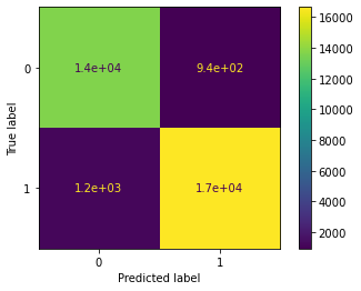
Precision and recall scores are both useful to evaluate the correct predictive capability of the model because they balance the false positives and false negatives inherent in prediction. The model shows a precision score of 0.948, suggesting the model is very good at predicting true positives. This means the model correctly predicts whether the airline passenger will be satisfied. The recall score of 0.940 is also very good. This means that the model does a good job of correctly identifying dissatisfied passengers within the dataset. These two metrics combined give a better assessment of model performance than the accuracy metric does alone.
The F1 score balances the precision and recall performance to give a combined assessment of how well this model delivers predictions. In this case, the F1 score is 0.944, which suggests very strong predictive power in this model.
Gain clarity with the confusion matrix
# Construct the confusion matrix for predicted and test values
cm = metrics.confusion_matrix(y_test, y_pred)

# Create the display for confusion matrix
disp = metrics.ConfusionMatrixDisplay(confusion_matrix=cm, display_labels=xgb_cv.classes_)

# Plot the visual in-line
disp.plot()
<sklearn.metrics._plot.confusion_matrix.ConfusionMatrixDisplay at 0x7f8c0dd82a10>
Visualize most important features
# Plot the relative feature importance of the predictor variables in the model
plot_importance(xgb_cv.best_estimator_)
<matplotlib.axes._subplots.AxesSubplot at 0x7f8c0bfa6ed0>
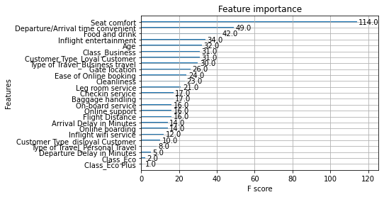
- By a wide margin, “seat comfort” rated as most important in the model.The type of seating is very different between first class and coach seating. However, the perks of being in first class also go beyond the seating type, so perhaps that is an underlying explanation of this feature’s importance.
- Surprisingly, delays (both arrival and departure) did not score as highly important.
Compare models
# Create a table of results to compare model performance
table = pd.DataFrame({'Model': ["Tuned Decision Tree", "Tuned Random Forest", "Tuned XGBoost"],
                      'F1': [0.945422, 0.947306, f1_score],
                      'Recall': [0.935863, 0.944501, rc_score],
                      'Precision': [0.955197, 0.950128, pc_score],
                      'Accuracy': [0.940864, 0.942450, ac_score]
                     }
                    )
table| Model | F1 | Recall | Precision | Accuracy | |
|---|---|---|---|---|---|
| 0 | Tuned Decision Tree | 0.945422 | 0.935863 | 0.955197 | 0.940864 |
| 1 | Tuned Random Forest | 0.947306 | 0.944501 | 0.950128 | 0.942450 |
| 2 | Tuned XGBoost | 0.939560 | 0.932717 | 0.946504 | 0.934031 |
Based on the results shown in the table above, the F1, precision, recall, and accuracy scores of the XGBoost model are similar to the corresponding scores of the decision tree and random forest models. The random forest model seemed to outperform the decision tree model as well as the XGBoost model.
Considerations
How could we share our findings with our team?
- Showcase the data used to create the prediction and the performance of the model overall.
- Review the sample output of the features and the confusion matrix to reference the model’s performance.
- Highlight the metric values, emphasizing the F1 score.
- Visualize the feature importance to showcase what drove the model’s predictions.
What could we share with and recommend to stakeholders?
- The model created is highly effective at predicting passenger satisfaction.
- The feature importance of seat comfort warrants additional investigation. It will be important to ask domain experts why they believe this feature scores so highly in this model.
Disclaimer: Like most of my posts, this content is intended solely for educational purposes and was created primarily for my personal reference. At times, I may rephrase original texts, and in some cases, I include materials such as graphs, equations, and datasets directly from their original sources.
I typically reference a variety of sources and update my posts whenever new or related information becomes available. For this particular post, the primary source was Google Advanced Data Analytics Professional Certificate program.