Introduction to the analysis of variance
So far we’ve seen
- Continuous and categorical variables.
- Linear regression, which can estimate continuous variables of interest.
- The chi squared goodness of fit test and test of independence, both examine the relationship between categorical variables.
Now we’ll focus on Analysis of Variance, which helps examine the relationship between categorical variables and continuous variables.
Analysis of Variance (ANOVA) is a group of statistical techniques that test the difference of means between three or more groups. ANOVA is an extension of t-tests. While t-tests examine the difference of means between two groups, ANOVA can test means between several groups.
ANOVA testing is useful when we want to test a hypothesis about group differences based on categorical independent variables. For example, if we wanted to determine whether changes in people’s weight when following different diets are statistically significant or due to chance, we could use ANOVA to analyze the results.
Imagine we’re wondering if different species of butterflies have different lifespans. ANOVA testing can help in this situation. There are two main types of ANOVA tests: One-way and two-way.
One-way ANOVA testing compares the means of one continuous dependent variable in three or more groups of one categorical variable.
Let’s say we want to study if butterfly lifespan is related to the species of the butterfly and the size of the butterfly. Now the data is varying according to two factors, species and size.
Null Hypothesis (H0): The means of each group are equal
Alternative Hypothesis (H1): The means of each group are not all equal
Two-way ANOVA testing compares the means of one continuous dependent variable based on two categorical variables. We are now testing three null hypothesis and alternative hypothesis statements at once:
| Null Hypothesis (H0) | Alternative Hypothesis (H1) | |
| Species | there is no difference in life spans between the three butterfly species | there is a difference in life spans between the three butterfly species |
| Size | there is no difference in life spans based on butterfly size | there is a difference in life spans based on butterfly size |
| Species & Size Interaction Effect | the effect of species on life span is independent of the butterfly size and vice versa | there is an interaction effect between butterfly size and species on life span |
Regression lets us understand how independent variables impact dependent variables. ANOVA allows us to zoom in on some of those relationships to tell a complete story by unpacking relationships in a pairwise fashion.
An overview of ANOVA
The intuition behind ANOVA is to compare the variability between different groups with the variability within the groups. If they are comparable, then the differences between groups are more likely to be due to sampling variability. On the other hand, if the variability between groups is much larger than the variability expected from the samples within their respective groups, then those groups are probably drawn from significantly different subpopulations.
The variation between groups and within groups is calculated as sums of squares, which are then expressed as a ratio. This ratio is known as the F-statistic.
Above we checked about one-way and two-way ANOVA. To review:
- One-way ANOVA: Compares the means of one continuous dependent variable based on three or more groups of one categorical variable.
- Two-way ANOVA: Compares the means of one continuous dependent variable based on three or more groups of two categorical variables.
One-way ANOVA
To understand the intuition behind ANOVA, let’s check a worked example of a simple one-way ANOVA test.
There are five steps in performing a one-way ANOVA test:
- Calculate group means and grand (overall) mean
- Calculate the sum of squares between groups (SSB) and the sum of squares within groups (SSW)
- Calculate mean squares for both SSB and SSW
- Compute the F-statistic
- Use the F-distribution and the F-statistic to get a p-value, which you use to decide whether to reject the null hypothesis
Example
Let’s imagine we have data of students studying for an exam. Suppose that in this case we wanted to compare three different studying programs (A, B, and C) to determine whether they have an effect on exam scores. Here is the data:
| Student | Study program (X) | Exam score (Y) |
| 1 | A | 88 |
| 2 | A | 79 |
| 3 | A | 86 |
| 4 | A | 90 |
| 5 | B | 94 |
| 6 | B | 84 |
| 7 | B | 87 |
| 8 | B | 89 |
| 9 | C | 85 |
| 10 | C | 76 |
| 11 | C | 81 |
| 12 | C | 78 |
First, we need to state our hypotheses:
H0: 𝜇A = 𝜇B = 𝜇C
The mean score of group A = the mean score of group B = the mean score of group C.
H1: NOT (𝜇A = 𝜇B = 𝜇C)
The means of each group are not all equal. Note that, even if only one mean differs, that is sufficient evidence to reject the null hypothesis.
Next, determine our confidence level—the threshold above which we will reject the null hypothesis. This value is dependent on our situation and usually requires some domain knowledge. A common threshold is 95%.
Step 1
Calculate group means and grand mean
The grand mean is the overall mean of all samples in all groups.
| Study program A scores | Study program B scores | Study program C scores |
| 88 | 94 | 85 |
| 79 | 84 | 76 |
| 86 | 87 | 81 |
| 90 | 89 | 78 |
| Mean: 85.75 | Mean: 88.5 | Mean: 80 |
Grand mean (MG) = 84.75
Step 2
A. Calculate the sum of squares between groups (SSB)
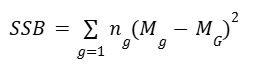
where:
ng = the number of samples in the gth group
Mg = mean of the gth group
MG = grand mean
→ SSB = [4(85.75 – 84.75)² + 4(88.5 – 84.75)² + 4(80 – 84.75)²]
= 4 + 56.25 + 90.25
= 150.5
B. Calculate the sum of squares within groups (SSW)
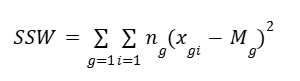
where:
xgi = sample i of the gth group
Mg = mean of the gth group
The double summation acts like a nested loop. The outer loop is for each group and the inner loop is for all the samples in that group. So this means,
- For each sample in group 1, subtract from it the group’s mean and square the result.
- Then, do the same thing with the samples in group 2, using the group 2 mean.
- Continue this way for all the groups and sum all the results.
| Program A | Program B | Program C | (xAi – MA)2 | (xBi – MB)2 | (xCi – MC)2 |
| 88 | 94 | 85 | 5.06 | 30.25 | 25 |
| 79 | 84 | 76 | 45.56 | 20.25 | 16 |
| 86 | 87 | 81 | 0.06 | 2.25 | 1 |
| 90 | 89 | 78 | 18.06 | 0.25 | 4 |
| MA = 85.75 | MB = 88.5 | MC = 80 | Sum: 68.75 | Sum: 53 | Sum: 46 |
→ SSW = 68.75 + 53 + 46
= 167.75
Step 3
Calculate mean squares between groups and within groups
The mean square is the sum of squares divided by the degrees of freedom, respectively.
A. Mean squares between groups (MSSB)
MSSB = SSB / k-1
where:
k = the number of groups
Note: k-1 represents the degrees of freedom between groups
→ MSSB = 150.5 / (3-1)
= 75.25
B. Mean squares within groups (MSSW)
MSSW = SSW / n-k
where:
n = the total number of samples in all groups
k = the number of groups
Note: n- k represents the degrees of freedom within groups
→ MSSW = 167.75 / (12-3)
= 18.64
Step 4
Compute the F-statistic
The F-statistic is the ratio of the mean sum of squares between groups (MSSB) to the mean sum of squares within groups (MSSW).
F-statistic = MSSB / MSSW
→ F-statistic = 75.25 / 18.64
= 4.04
A higher F-statistic indicates a greater variability between group means relative to the variability within groups, suggesting that at least one group mean is significantly different from the others.
Step 5
Use the F-distribution and the F-statistic to get a p-value,
which we use to decide whether to reject the null hypothesis.
Similar to t-tests and 𝛸2 tests, ANOVA testing finds the area under a particular probability distribution curve, the F-distribution, of the null hypothesis to determine a p-value. The larger the F-statistic, the lesser the area beneath the curve and the more evidence against the null hypothesis, thus resulting in a lower p-value.
The shape of the F-distribution curve is determined by the degrees of freedom between and within groups. Below is a graph depicting F-distributions for three, five, and 10 groups, each group containing 50 samples.
Note that “dfn” represents the degrees of freedom in the numerator (between groups) and “dfd” represents the degrees of freedom in the denominator (within groups). Notice how the degrees of freedom affect the shape of the curve.

Similar to 𝛸2 curves, F-distributions help determine the probability of falsely rejecting the null hypothesis. In the case of ANOVA, this probability is represented by the area of the F-distribution beneath the curve where x ≥ our F-statistic.
For example, the following graph depicts the F-distribution for the exam scores example. It has two degrees of freedom in the numerator and nine degrees of freedom in the denominator. The area beneath the curve where x ≥ 4.04 (the computed F-statistic) is shaded.

We can use statistical software to calculate this area. In this case, the area beneath the F-distribution to the right of 4.04 is 0.05604. This is the probability of observing an F-statistic greater than 4.04 if the null hypothesis were true. Whether this is sufficient to reject the null hypothesis is a decision we make at the beginning of our hypothesis test.
For example, if we decided that we wanted a confidence level of 95% or greater, we cannot reject the null hypothesis that the means of the distributions for each program of study are all the same, because the p-value is 0.056.
Assumptions of ANOVA
ANOVA will only work if the following assumptions are true:
- The dependent values for each group come from normal distributions.
- Note that this assumption does NOT mean that all of the dependent values, taken together, must be normally distributed. Instead, it means that within each group, the dependent values should be normally distributed.
- ANOVA is generally robust to violations of normality, especially when sample sizes are large or similar across groups, due to the central limit theorem. However, significant violations can lead to incorrect conclusions.
- The variances across groups are equal.
- ANOVA compares means across groups and assumes that the variance around these means is the same for all groups. If the variances are unequal (i.e., heteroscedastic), it could lead to incorrect conclusions.
- Observations are independent of each other.
- ANOVA assumes that one observation does not influence or predict any other observation. If there is autocorrelation among the observations, the results of the ANOVA test could be biased.
Key takeaways
- ANOVA tests are statistical tests that examine whether or not the means of a continuous dependent variable are significantly different from one another based on the different levels of one or more independent categorical variables.
- It is sufficient for one group’s mean to be significantly different from the others to reject the null hypothesis; however, ANOVA testing is limited in that it doesn’t tell us which group is different. To make such a determination, other tests are necessary.
- ANOVA works by comparing the variance between each group to the variance within each group. The greater the ratio of variance between groups to variance within groups, the greater the likelihood of rejecting the null hypothesis.
- ANOVA depends on certain assumptions, so it is important to check that our data meets them in order to avoid drawing false conclusions. At the very least, if our data does not meet all of them, we need to identify these violations.
Disclaimer: Like most of my posts, this content is intended solely for educational purposes and was created primarily for my personal reference. At times, I may rephrase original texts, and in some cases, I include materials such as graphs, equations, and datasets directly from their original sources.
I typically reference a variety of sources and update my posts whenever new or related information becomes available. For this particular post, the primary source was Google Advanced Data Analytics Professional Certificate.