Introduction
For this activity, we work as a consultant for an airline. The airline is interested in predicting whether a future customer would be satisfied with their services given previous customer feedback about their flight experience. The airline would like us to construct and evaluate a model that can accomplish this goal. Specifically, they are interested in knowing which features are most important to customer satisfaction.
The data for this activity includes survey responses from 129,880 customers. It includes data points such as class, flight distance, and in-flight entertainment, among others. In a previous activity, we utilized a binomial logistic regression model to help the airline better understand this data. In this activity, our goal will be to utilize a decision tree model to predict whether or not a customer will be satisfied with their flight experience.
Because this activity uses a dataset from the industry, we will need to conduct basic EDA, data cleaning, and other manipulations to prepare the data for modeling.
Step 1: Import and Load
# Standard operational package imports
import numpy as np
import pandas as pd

# Important imports for modeling and evaluation
from sklearn.model_selection import train_test_split
from sklearn.model_selection import GridSearchCV
from sklearn.tree import DecisionTreeClassifier
from sklearn.tree import plot_tree
import sklearn.metrics as metrics

# Visualization package imports
import matplotlib.pyplot as plt
import seaborn as sns
df_original = pd.read_csv("Invistico_Airline.csv")
df_original.head(n = 10)
| satisfaction | Customer Type | Age | Type of Travel | Class | Flight Distance | Seat comfort | Departure/Arrival time convenient | Food and drink | Gate location | … | Online support | Ease of Online booking | On-board service | Leg room service | Baggage handling | Checkin service | Cleanliness | Online boarding | Departure Delay in Minutes | Arrival Delay in Minutes | |
|---|---|---|---|---|---|---|---|---|---|---|---|---|---|---|---|---|---|---|---|---|---|
| 0 | satisfied | Loyal Customer | 65 | Personal Travel | Eco | 265 | 0 | 0 | 0 | 2 | … | 2 | 3 | 3 | 0 | 3 | 5 | 3 | 2 | 0 | 0.0 |
| 1 | satisfied | Loyal Customer | 47 | Personal Travel | Business | 2464 | 0 | 0 | 0 | 3 | … | 2 | 3 | 4 | 4 | 4 | 2 | 3 | 2 | 310 | 305.0 |
| 2 | satisfied | Loyal Customer | 15 | Personal Travel | Eco | 2138 | 0 | 0 | 0 | 3 | … | 2 | 2 | 3 | 3 | 4 | 4 | 4 | 2 | 0 | 0.0 |
| 3 | satisfied | Loyal Customer | 60 | Personal Travel | Eco | 623 | 0 | 0 | 0 | 3 | … | 3 | 1 | 1 | 0 | 1 | 4 | 1 | 3 | 0 | 0.0 |
| 4 | satisfied | Loyal Customer | 70 | Personal Travel | Eco | 354 | 0 | 0 | 0 | 3 | … | 4 | 2 | 2 | 0 | 2 | 4 | 2 | 5 | 0 | 0.0 |
| 5 | satisfied | Loyal Customer | 30 | Personal Travel | Eco | 1894 | 0 | 0 | 0 | 3 | … | 2 | 2 | 5 | 4 | 5 | 5 | 4 | 2 | 0 | 0.0 |
| 6 | satisfied | Loyal Customer | 66 | Personal Travel | Eco | 227 | 0 | 0 | 0 | 3 | … | 5 | 5 | 5 | 0 | 5 | 5 | 5 | 3 | 17 | 15.0 |
| 7 | satisfied | Loyal Customer | 10 | Personal Travel | Eco | 1812 | 0 | 0 | 0 | 3 | … | 2 | 2 | 3 | 3 | 4 | 5 | 4 | 2 | 0 | 0.0 |
| 8 | satisfied | Loyal Customer | 56 | Personal Travel | Business | 73 | 0 | 0 | 0 | 3 | … | 5 | 4 | 4 | 0 | 1 | 5 | 4 | 4 | 0 | 0.0 |
| 9 | satisfied | Loyal Customer | 22 | Personal Travel | Eco | 1556 | 0 | 0 | 0 | 3 | … | 2 | 2 | 2 | 4 | 5 | 3 | 4 | 2 | 30 | 26.0 |
10 rows × 22 columns
Step 2: Data exploration, data cleaning, and model preparation
We’ll prepare the data to be suitable for decision tree classifiers. This includes:
- Exploring the data
- Checking for missing values
- Encoding the data
- Renaming a column
- Creating the training and testing data
Explore the data
df_original.dtypessatisfaction object Customer Type object Age int64 Type of Travel object Class object Flight Distance int64 Seat comfort int64 Departure/Arrival time convenient int64 Food and drink int64 Gate location int64 Inflight wifi service int64 Inflight entertainment int64 Online support int64 Ease of Online booking int64 On-board service int64 Leg room service int64 Baggage handling int64 Checkin service int64 Cleanliness int64 Online boarding int64 Departure Delay in Minutes int64 Arrival Delay in Minutes float64 dtype: object
Output unique values
The Class column is ordinal (meaning there is an inherent order that is significant). For example, airlines typically charge more for ‘Business’ than ‘Eco Plus’ and ‘Eco’.
df_original["Class"].unique()array(['Eco', 'Business', 'Eco Plus'], dtype=object)
Check the counts of the predicted labels
In order to predict customer satisfaction, we need to verify if the dataset is imbalanced.
df_original['satisfaction'].value_counts(dropna = False)satisfied 71087 dissatisfied 58793 Name: satisfaction, dtype: int64
54.7 percent (71087/129880) of customers were satisfied. This value can be compared to a decision tree’s model accuracy.
Check for missing values
The sklearn decision tree implementation does not support missing values.
df_original.isnull().sum()satisfaction 0 Customer Type 0 Age 0 Type of Travel 0 Class 0 Flight Distance 0 Seat comfort 0 Departure/Arrival time convenient 0 Food and drink 0 Gate location 0 Inflight wifi service 0 Inflight entertainment 0 Online support 0 Ease of Online booking 0 On-board service 0 Leg room service 0 Baggage handling 0 Checkin service 0 Cleanliness 0 Online boarding 0 Departure Delay in Minutes 0 Arrival Delay in Minutes 393 dtype: int64
Check the number of rows and columns in the dataset
df_original.shape(129880, 22)
Drop the rows with missing values
df_subset = df_original.dropna(axis=0).reset_index(drop = True)
# Check for missing values
df_subset.isna().sum()
satisfaction 0 Customer Type 0 Age 0 Type of Travel 0 Class 0 Flight Distance 0 Seat comfort 0 Departure/Arrival time convenient 0 Food and drink 0 Gate location 0 Inflight wifi service 0 Inflight entertainment 0 Online support 0 Ease of Online booking 0 On-board service 0 Leg room service 0 Baggage handling 0 Checkin service 0 Cleanliness 0 Online boarding 0 Departure Delay in Minutes 0 Arrival Delay in Minutes 0 dtype: int64
Encode the data
Four columns (satisfaction, Customer Type, Type of Travel, Class) are the pandas dtype object. Decision trees need numeric columns.
df_subset['Class'] = df_subset['Class'].map({"Business": 3, "Eco Plus": 2, "Eco": 1}) Represent the data in the target variable numerically
To represent the data in the target variable numerically, we’ll assign "satisfied" to the label 1 and "dissatisfied" to the label 0 in the satisfaction column.
df_subset['satisfaction'] = df_subset['satisfaction'].map({"satisfied": 1, "dissatisfied": 0})Convert categorical columns into numeric
There are other columns in the dataset that are still categorical. We need to convert them too.
df_subset = pd.get_dummies(df_subset, drop_first = True)Check column data types
Now that we have converted categorical columns into numeric, let’s check our column data types.
df_subset.dtypessatisfaction int64 Age int64 Class int64 Flight Distance int64 Seat comfort int64 Departure/Arrival time convenient int64 Food and drink int64 Gate location int64 Inflight wifi service int64 Inflight entertainment int64 Online support int64 Ease of Online booking int64 On-board service int64 Leg room service int64 Baggage handling int64 Checkin service int64 Cleanliness int64 Online boarding int64 Departure Delay in Minutes int64 Arrival Delay in Minutes float64 Customer Type_disloyal Customer uint8 Type of Travel_Personal Travel uint8 dtype: object
Create the training and testing data
y = df_subset["satisfaction"]

X = df_subset.copy()
X = X.drop("satisfaction", axis = 1)

X_train, X_test, y_train, y_test = train_test_split(X, y, test_size=0.25, random_state=0)
Step 3: Model building
decision_tree = DecisionTreeClassifier(random_state=0)

decision_tree.fit(X_train, y_train)

dt_pred = decision_tree.predict(X_test)
Decision trees require no assumptions regarding the distribution of underlying data and don’t require scaling of features.
Step 4: Results and evaluation
print("Decision Tree")
print("Accuracy:", "%.6f" % metrics.accuracy_score(y_test, dt_pred))
print("Precision:", "%.6f" % metrics.precision_score(y_test, dt_pred))
print("Recall:", "%.6f" % metrics.recall_score(y_test, dt_pred))
print("F1 Score:", "%.6f" % metrics.f1_score(y_test, dt_pred))
Decision Tree
Accuracy: 0.935438
Precision: 0.942859
Recall: 0.939030
F1 Score: 0.940940
Decision trees can be particularly susceptible to overfitting. Combining hyperparameter tuning and grid search can help ensure this doesn’t happen. For instance, setting an appropriate value for max depth could potentially help reduce a decision tree’s overfitting problem by limiting how deep a tree can grow.
Produce a confusion matrix
cm = metrics.confusion_matrix(y_test, dt_pred, labels = decision_tree.classes_)
disp = metrics.ConfusionMatrixDisplay(confusion_matrix = cm,display_labels = decision_tree.classes_)
disp.plot()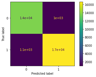
- In the confusion matrix, there are a high proportion of true positives and true negatives (where the matrix accurately predicted that the customer would be satisfied or dissatified, respectively).
- The matrix also had a relatively low number of false positives and false negatives (where the matrix innacurately predicted that the customer would be satisfied or dissatified, respectively.)
Plot the decision tree
plt.figure(figsize=(20,12))
plot_tree(decision_tree, max_depth=2, fontsize=14, feature_names=X.columns)
Calculate feature importance
The DecisionTreeClassifier class comes with a feature_importances_ attribute that provides access to the features’ relative importance in the model. The feature importance is computed when the fit() method is called on the DecisionTreeClassifier instance. In other words, it’s information that is generated during model training.
How the feature importance works
For each feature used in the tree, the algorithm finds all of the decision nodes that use that particular feature as the split criterion. Then for each of those decision nodes it computes the decrease in Gini impurity (or entropy, or log loss, or whatever metric we select when we fit the model; default is Gini impurity) that results from that split (so, the decrease from parent to children). Then the algorithm sums up the decreases across all the decisions made using that feature and expresses it as a percentage of the total decrease that resulted from all features.
Here is a simple example of how we can calculate feature importance from a tree diagram. This tree splits 10 samples using two features, X1 and X2:
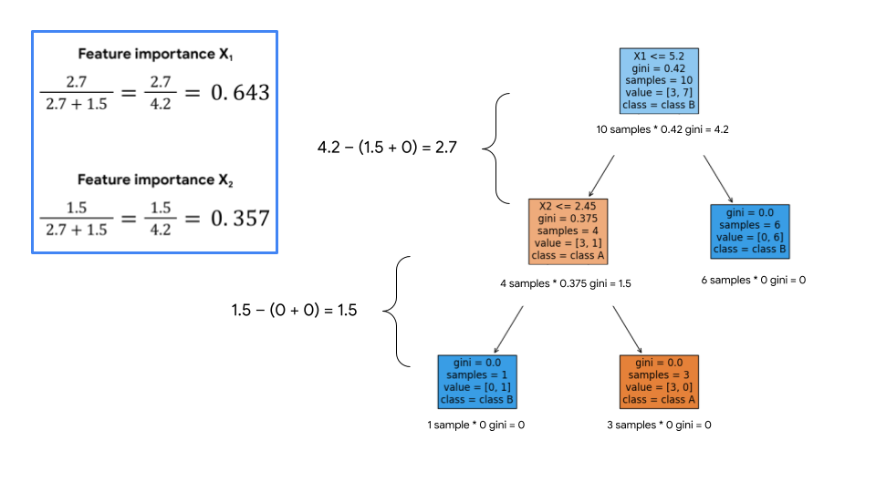
Notice that the reduction in Gini impurity is weighted based on how many samples are in each node. Ultimately, the reduction that results from each feature is normalized (i.e., expressed as a percentage), and this percentage represents the importance of a given feature.
This can be interpreted as: X1 is responsible for 64.3% of the overall reduction of Gini impurity in the model, and X2 is responsible for 35.7% of the overall reduction of Gini impurity in the model.
Plotting the feature importance
Using the feature_importances_ attribute to fetch the relative importances of each feature, we can then plot the results.
importances = decision_tree.feature_importances_

forest_importances = pd.Series(importances, index=X.columns).sort_values(ascending=False)

fig, ax = plt.subplots()
forest_importances.plot.bar(ax=ax)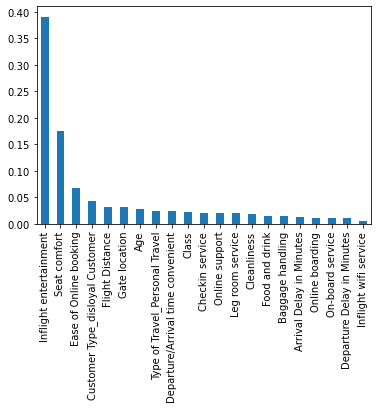
The feature importance graph seems to confirm that 'Inflight entertainment', 'Seat comfort', and 'Ease of Online booking' are the most important features for this model.
Hyperparameter tuning
Knowing how and when to adjust or tune a model can help a data professional significantly increase performance. Here we will find the best values for the hyperparameters max_depth and min_samples_leaf using grid search and cross validation.
tree_para = {'max_depth':[1,2,3,4,5,6,7,8,9,10,11,12,13,14,15,16,17,18,19,20,30,40,50],
             'min_samples_leaf': [2,3,4,5,6,7,8,9, 10, 15, 20, 50]}

scoring = {'accuracy', 'precision', 'recall', 'f1'}
Check combinations of values
Note: The cell below may take up to 15 minutes to run.
tuned_decision_tree = DecisionTreeClassifier(random_state=0)

clf = GridSearchCV(tuned_decision_tree,
                   tree_para,
                   scoring = scoring,
                   cv=5,
                   refit="f1")

clf.fit(X_train, y_train)
GridSearchCV(cv=5, error_score=nan,
estimator=DecisionTreeClassifier(ccp_alpha=0.0, class_weight=None,
criterion='gini', max_depth=None,
max_features=None,
max_leaf_nodes=None,
min_impurity_decrease=0.0,
min_impurity_split=None,
min_samples_leaf=1,
min_samples_split=2,
min_weight_fraction_leaf=0.0,
presort='deprecated',
random_state=0, splitter='best'),
iid='deprecated', n_jobs=None,
param_grid={'max_depth': [1, 2, 3, 4, 5, 6, 7, 8, 9, 10, 11, 12,
13, 14, 15, 16, 17, 18, 19, 20, 30, 40,
50],
'min_samples_leaf': [2, 3, 4, 5, 6, 7, 8, 9, 10, 15,
20, 50]},
pre_dispatch='2*n_jobs', refit='f1', return_train_score=False,
scoring={'f1', 'recall', 'precision', 'accuracy'}, verbose=0)
Compute the best combination of values for the hyperparameters
clf.best_estimator_DecisionTreeClassifier(ccp_alpha=0.0, class_weight=None, criterion='gini',
max_depth=18, max_features=None, max_leaf_nodes=None,
min_impurity_decrease=0.0, min_impurity_split=None,
min_samples_leaf=2, min_samples_split=2,
min_weight_fraction_leaf=0.0, presort='deprecated',
random_state=0, splitter='best')
After running the DecisionTreeClassifier, the maximum depth is 18 and the minimum number of samples is 2, meaning this is the best combination of values.
Determine the best average validation score
print("Best Avg. Validation Score: ", "%.4f" % clf.best_score_)Best Avg. Validation Score: 0.9454
Determine the “best” decision tree model’s accuracy, precision, recall, and F1 score
results = pd.DataFrame(columns=['Model', 'F1', 'Recall', 'Precision', 'Accuracy'])

def make_results(model_name, model_object):
    """
    Accepts as arguments a model name (your choice - string) and
    a fit GridSearchCV model object.
    Returns a pandas df with the F1, recall, precision, and accuracy scores
    for the model with the best mean F1 score across all validation folds.
    """
    # Get all the results from the CV and put them in a df.
    cv_results = pd.DataFrame(model_object.cv_results_)

    # Isolate the row of the df with the max(mean f1 score).
    best_estimator_results = cv_results.iloc[cv_results['mean_test_f1'].idxmax(), :]

    # Extract accuracy, precision, recall, and f1 score from that row.
    f1 = best_estimator_results.mean_test_f1
    recall = best_estimator_results.mean_test_recall
    precision = best_estimator_results.mean_test_precision
    accuracy = best_estimator_results.mean_test_accuracy

    # Create table of results
    table = pd.DataFrame({'Model': [model_name],
                          'F1': [f1],
                          'Recall': [recall],
                          'Precision': [precision],
                          'Accuracy': [accuracy]
                         }
                        )

    return table

result_table = make_results("Tuned Decision Tree", clf)

result_table| Model | F1 | Recall | Precision | Accuracy | |
|---|---|---|---|---|---|
| 0 | Tuned Decision Tree | 0.945422 | 0.935863 | 0.955197 | 0.940864 |
The F1 score for the decision tree that was not hyperparameter tuned is 0.940940 and the F1 score for the hyperparameter-tuned decision tree is 0.945422. While ensuring that overfitting doesn’t occur is necessary for some models, it didn’t make a meaningful difference in improving this model.
Plot the “best” decision tree
Use the plot_tree function to produce a representation of the tree to pinpoint where the splits in the data are occurring. This will allow us to review the “best” decision tree.
plt.figure(figsize=(20,12))
plot_tree(clf.best_estimator_, max_depth=2, fontsize=14, feature_names=X.columns)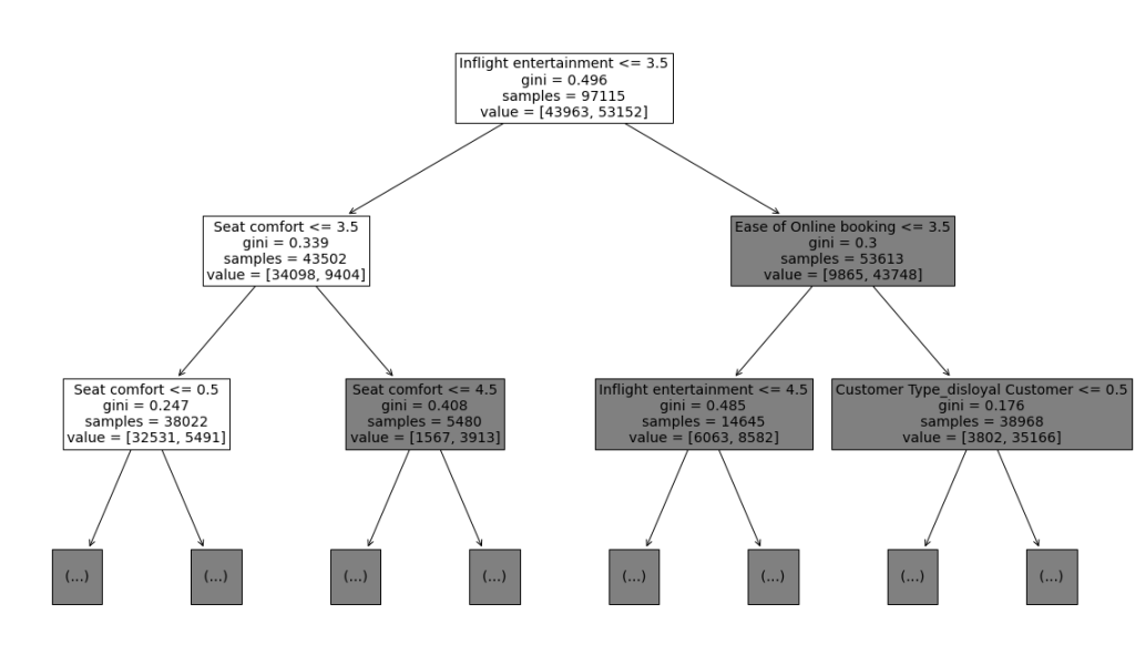
The plot makes it seem like 'Inflight entertainment', 'Seat comfort', and 'Ease of Online booking' are among the most important features. The code below outputs a “most important” features graph from the model.
Build another feature importance graph
importances = clf.best_estimator_.feature_importances_

forest_importances = pd.Series(importances, index=X.columns).sort_values(ascending=False)

fig, ax = plt.subplots()
forest_importances.plot.bar(ax=ax)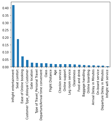
The feature importance graph seems to confirm that 'Inflight entertainment', 'Seat comfort', and 'Ease of Online booking' are the “most important” features for this model.
What is the most important metric in this business case?
Any of the metrics in this business case could be considered important, depending on what the stakeholder or domain expert cares about. The following are reasons why each metric is important:
- Accuracy tends to be the metric that the stakeholders can best understand.
- Precision measures what proportion of predicted positives is truly positive. For example, if we wanted to not falsely claiming a customer is satisfied, precision would be a good metric. Assuming a customer is happy when they are really not might lead to customer churn.
- Recall measures the percentage of actual positives a model correctly identified (true positive). For this dataset, the airline might want to limit false negatives (actually satisfied people who are predicted to be unsatisfied). Assuming a customer is unhappy when the customer is happy can lead to the airline wasting resources trying to improve the customer experience of an already happy customer.
- F1 balances precision and recall. It is the harmonic mean of precision and recall, or their product divided by their sum.
Considerations
What could we recommend to stakeholders?
- Customer satisfaction is highly tied to
'Inflight entertainment','Seat comfort', and'Ease of Online booking'. Improving these experiences should lead to better customer satisfaction. - The success of the model suggests that the airline should invest more effort into model building and model understanding since this model seemed to be very good at predicting customer satisfaction.
Disclaimer: Like most of my posts, this content is intended solely for educational purposes and was created primarily for my personal reference. At times, I may rephrase original texts, and in some cases, I include materials such as graphs, equations, and datasets directly from their original sources.
I typically reference a variety of sources and update my posts whenever new or related information becomes available. For this particular post, the primary source was Google Advanced Data Analytics Professional Certificate program.