Introduction
In this activity, we are a consultant for a scientific organization that works to support and sustain penguin colonies. We are tasked with helping other staff members learn more about penguins in order to achieve this mission.
The data for this activity is in a spreadsheet that includes datapoints across a sample size of 345 penguins, such as species, island, and sex. We will use a K-means clustering model to group this data and identify patterns that provide important insights about penguins.
Step 1: Imports
# Import standard operational packages.
import numpy as np
import pandas as pd

# Important tools for modeling and evaluation.
from sklearn.cluster import KMeans
from sklearn.metrics import silhouette_score
from sklearn.preprocessing import StandardScaler

# Import visualization packages.
import matplotlib.pyplot as plt
import seaborn as sns
# Save the `pandas` DataFrame in variable `penguins`
penguins = pd.read_csv("penguins.csv")# Review the first 10 rows
penguins.head(n = 10)| species | island | bill_length_mm | bill_depth_mm | flipper_length_mm | body_mass_g | sex | |
|---|---|---|---|---|---|---|---|
| 0 | Adelie | Torgersen | 39.1 | 18.7 | 181.0 | 3750.0 | male |
| 1 | Adelie | Torgersen | 39.5 | 17.4 | 186.0 | 3800.0 | female |
| 2 | Adelie | Torgersen | 40.3 | 18.0 | 195.0 | 3250.0 | female |
| 3 | Adelie | Torgersen | NaN | NaN | NaN | NaN | NaN |
| 4 | Adelie | Torgersen | 36.7 | 19.3 | 193.0 | 3450.0 | female |
| 5 | Adelie | Torgersen | 39.3 | 20.6 | 190.0 | 3650.0 | male |
| 6 | Adelie | Torgersen | 38.9 | 17.8 | 181.0 | 3625.0 | female |
| 7 | Adelie | Torgersen | 39.2 | 19.6 | 195.0 | 4675.0 | male |
| 8 | Adelie | Torgersen | 34.1 | 18.1 | 193.0 | 3475.0 | NaN |
| 9 | Adelie | Torgersen | 42.0 | 20.2 | 190.0 | 4250.0 | NaN |
Step 2: Data exploration
After loading the dataset, the next step is to prepare the data to be suitable for clustering. This includes:
- Exploring data
- Checking for missing values
- Encoding data
- Dropping a column
- Scaling the features using
StandardScaler
Explore data
To cluster penguins of multiple different species, we need to determine how many different types of penguin species are in the dataset.
# Find out how many penguin types there are
penguins['species'].unique()
array(['Adelie', 'Chinstrap', 'Gentoo'], dtype=object)
# Find the count of each species type
penguins['species'].value_counts(dropna = False)
Adelie 152 Gentoo 124 Chinstrap 68 Name: species, dtype: int64
- There are three types of species. Note the Chinstrap species is less common than the other species. This has a chance to affect K-means clustering as K-means performs best with similar sized groupings.
- For purposes of clustering, we’ll pretend we don’t know that there are three different types of species. Then, we can explore whether the algorithm can discover the different species. We might even find other relationships in the data.
Check for missing values
An assumption of K-means is that there are no missing values.
# Check for missing values
penguins.isnull().sum()
species 0 island 0 bill_length_mm 2 bill_depth_mm 2 flipper_length_mm 2 body_mass_g 2 sex 11 dtype: int64
Now, we’ll drop the rows with missing values and save the resulting pandas DataFrame in a variable named penguins_subset.
# Drop rows with missing values
# Save DataFrame in variable `penguins_subset`
penguins_subset = penguins.dropna(axis=0).reset_index(drop = True)
# Check for missing values
penguins_subset.isna().sum()species 0 island 0 bill_length_mm 0 bill_depth_mm 0 flipper_length_mm 0 body_mass_g 0 sex 0 dtype: int64
# View first 10 rows
penguins_subset.head(10)| species | island | bill_length_mm | bill_depth_mm | flipper_length_mm | body_mass_g | sex | |
|---|---|---|---|---|---|---|---|
| 0 | Adelie | Torgersen | 39.1 | 18.7 | 181.0 | 3750.0 | male |
| 1 | Adelie | Torgersen | 39.5 | 17.4 | 186.0 | 3800.0 | female |
| 2 | Adelie | Torgersen | 40.3 | 18.0 | 195.0 | 3250.0 | female |
| 3 | Adelie | Torgersen | 36.7 | 19.3 | 193.0 | 3450.0 | female |
| 4 | Adelie | Torgersen | 39.3 | 20.6 | 190.0 | 3650.0 | male |
| 5 | Adelie | Torgersen | 38.9 | 17.8 | 181.0 | 3625.0 | female |
| 6 | Adelie | Torgersen | 39.2 | 19.6 | 195.0 | 4675.0 | male |
| 7 | Adelie | Torgersen | 41.1 | 17.6 | 182.0 | 3200.0 | female |
| 8 | Adelie | Torgersen | 38.6 | 21.2 | 191.0 | 3800.0 | male |
| 9 | Adelie | Torgersen | 34.6 | 21.1 | 198.0 | 4400.0 | male |
Encode data
Some versions of the penguins dataset have values encoded in the sex column as ‘Male’ and ‘Female’ instead of ‘MALE’ and ‘FEMALE’. The code below will make sure all values are ALL CAPS.
penguins_subset['sex'] = penguins_subset['sex'].str.upper()K-means needs numeric columns for clustering. We’ll convert the categorical column 'sex' into numeric. There is no need to convert the 'species' column because it isn’t being used as a feature in the clustering algorithm.
# Convert `sex` column from categorical to numeric
penguins_subset = pd.get_dummies(penguins_subset, drop_first = True, columns=['sex'])
Drop a column
Drop the categorical column island from the dataset. While it has value, this notebook is trying to confirm if penguins of the same species exhibit different physical characteristics based on sex. This doesn’t include location.
Note that the 'species' column is not numeric. We woon’t drop the 'species' column for now. It could potentially be used to help understand the clusters later.
# Drop the island column
penguins_subset = penguins_subset.drop(['island'], axis=1)
Scale the features
Because K-means uses distance between observations as its measure of similarity, it’s important to scale the data before modeling. StandardScaler scales each point xᵢ by subtracting the mean observed value for that feature and dividing by the standard deviation:
x-scaled = (xᵢ – mean(X)) / σ
This ensures that all variables have a mean of 0 and variance/standard deviation of 1.
Note: Because the species column isn’t a feature, it doesn’t need to be scaled.
First, we’ll copy all the features except the 'species' column to a DataFrame X.
# Exclude `species` variable from X
X = penguins_subset.drop(['species'], axis=1)
#Scale the features
#Assign the scaled data to variable `X_scaled`
X_scaled = StandardScaler().fit_transform(X)Step 3: Data modeling
Now, we’ll fit K-means and evaluate inertia for different values of k. Because we may not know how many clusters exist in the data, we’ll start by fitting K-means and examining the inertia values for different values of k. To do this, we’ll write a function called kmeans_inertia that takes in num_clusters and x_vals (X_scaled) and returns a list of each k-value’s inertia.
# Fit K-means and evaluate inertia for different values of k
num_clusters = [i for i in range(2, 11)]

def kmeans_inertia(num_clusters, x_vals):
    """
    Accepts as arguments list of ints and data array.
    Fits a KMeans model where k = each value in the list of ints.
    Returns each k-value's inertia appended to a list.
    """
    inertia = []
    for num in num_clusters:
        kms = KMeans(n_clusters=num, random_state=42)
        kms.fit(x_vals)
        inertia.append(kms.inertia_)

    return inertia
# Return a list of inertia for k=2 to 10
inertia = kmeans_inertia(num_clusters, X_scaled)
inertia[885.6224143652249, 578.8284278107235, 386.14534424773285, 284.5464837898288, 217.92858573807678, 201.39287843423264, 186.82270634899209, 173.47283154242746, 164.55854201979943]
Next, we’ll create a line plot that shows the relationship between num_clusters and inertia.
# Create a line plot
plot = sns.lineplot(x=num_clusters, y=inertia, marker = 'o')
plot.set_xlabel("Number of clusters")
plot.set_ylabel("Inertia")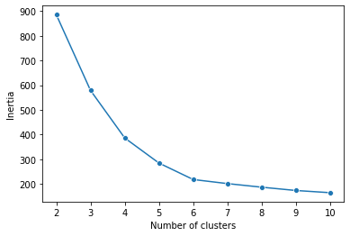
The plot seems to depict an elbow at six clusters, but there isn’t a clear method for confirming that a six-cluster model is optimal. Therefore, the silhouette scores should be checked.
Step 4: Results and evaluation
Now, we’ll evaluate the silhouette score using the silhouette_score() function. Silhouette scores are used to study the distance between clusters.
Then, we’ll compare the silhouette score of each value of k, from 2 through 10. To do this, we’ll write a function called kmeans_sil that takes in num_clusters and x_vals (X_scaled) and returns a list of each k-value’s silhouette score.
# Evaluate silhouette score
# Write a function to return a list of each k-value's score
def kmeans_sil(num_clusters, x_vals):
    """
    Accepts as arguments list of ints and data array.
    Fits a KMeans model where k = each value in the list of ints.
    Calculates a silhouette score for each k value.
    Returns each k-value's silhouette score appended to a list.
    """
    sil_score = []
    for num in num_clusters:
        kms = KMeans(n_clusters=num, random_state=42)
        kms.fit(x_vals)
        sil_score.append(silhouette_score(x_vals, kms.labels_))

    return sil_score

sil_score = kmeans_sil(num_clusters, X_scaled)
sil_score
[0.44398088353055243, 0.45101024097188364, 0.5080140996630784, 0.519998574860868, 0.5263224884981607, 0.47774022332151733, 0.42680523270292947, 0.35977478703657334, 0.3589883410610364]
Next, we’ll create a line plot that shows the relationship between num_clusters and sil_score.
# Create a line plot
plot = sns.lineplot(x=num_clusters, y=sil_score, marker = 'o')
plot.set_xlabel("# of clusters")
plot.set_ylabel("Silhouette Score")
Silhouette scores near 1 indicate that samples are far away from neighboring clusters. Scores close to 0 indicate that samples are on or very close to the decision boundary between two neighboring clusters.
The plot indicates that the silhouette score is closest to 1 when the data is partitioned into six clusters, although five clusters also yield a relatively good silhouette score.
Optimal k-value
To decide on an optimal k-value, we’ll fit a six-cluster model to the dataset.
# Fit a 6-cluster model
kmeans6 = KMeans(n_clusters=6, random_state=42)
kmeans6.fit(X_scaled)
KMeans(algorithm='auto', copy_x=True, init='k-means++', max_iter=300,
n_clusters=6, n_init=10, n_jobs=None, precompute_distances='auto',
random_state=42, tol=0.0001, verbose=0)
# Print unique labels
print('Unique labels:', np.unique(kmeans6.labels_))
Unique labels: [0 1 2 3 4 5]
Now, we’ll create a new column cluster that indicates cluster assignment in the DataFrame penguins_subset. It’s important to understand the meaning of each cluster’s labels, then we’ll decide whether the clustering makes sense.
Note: This task is done using penguins_subset because it is often easier to interpret unscaled data.
# Create a new column `cluster`
penguins_subset['cluster'] = kmeans6.labels_
penguins_subset.head()| species | bill_length_mm | bill_depth_mm | flipper_length_mm | body_mass_g | sex_MALE | cluster | |
|---|---|---|---|---|---|---|---|
| 0 | Adelie | 39.1 | 18.7 | 181.0 | 3750.0 | 1 | 0 |
| 1 | Adelie | 39.5 | 17.4 | 186.0 | 3800.0 | 0 | 2 |
| 2 | Adelie | 40.3 | 18.0 | 195.0 | 3250.0 | 0 | 2 |
| 3 | Adelie | 36.7 | 19.3 | 193.0 | 3450.0 | 0 | 2 |
| 4 | Adelie | 39.3 | 20.6 | 190.0 | 3650.0 | 1 | 0 |
Let’s use groupby to verify if any 'cluster' can be differentiated by 'species'.
# Verify if any `cluster` can be differentiated by `species`
penguins_subset.groupby(by=['cluster', 'species']).size()
cluster species
0 Adelie 71
1 Gentoo 58
2 Adelie 73
Chinstrap 5
3 Gentoo 61
4 Adelie 2
Chinstrap 34
5 Chinstrap 29
dtype: int64
Next, we’ll interpret the groupby outputs. Although the results of the groupby show that each 'cluster' can be differentiated by 'species', it is useful to visualize these results. The graph shows that each 'cluster' can be differentiated by 'species'.
penguins_subset.groupby(by=['cluster', 'species']).size().plot.bar(title='Clusters differentiated by species',
            figsize=(6, 5),
            ylabel='Size',
            xlabel='(Cluster, Species)')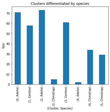
Now let’s use groupby to verify if each 'cluster' can be differentiated by 'species' AND 'sex_MALE'.
# Verify if each `cluster` can be differentiated by `species` AND `sex_MALE`
penguins_subset.groupby(by=['cluster','species', 'sex_MALE']).size().sort_values(ascending = False)
cluster species sex_MALE 2 Adelie 0 73 0 Adelie 1 71 3 Gentoo 1 61 1 Gentoo 0 58 4 Chinstrap 1 34 5 Chinstrap 0 29 2 Chinstrap 0 5 4 Adelie 1 2 dtype: int64
- Even though clusters 1 and 3 weren’t all one species or sex, the
groupbyindicates that the algorithm produced clusters mostly differentiated by species and sex.
Finally, let’s interpret the groupby outputs and visualize these results. The graph shows that each 'cluster' can be differentiated by 'species' and 'sex_MALE'. Furthermore, each cluster is mostly comprised of one sex and one species.
penguins_subset.groupby(by=['cluster','species','sex_MALE']).size().unstack(level = 'species', fill_value=0).plot.bar(title='Clusters differentiated by species and sex',                                                                                                                     figsize=(6, 5),                                                                                                                     ylabel='Size',                                                                                                                    xlabel='(Cluster, Sex)')
plt.legend(bbox_to_anchor=(1.3, 1.0))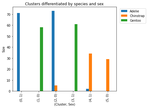
Considerations
Here are some key takeaways:
- Many machine learning workflows are about cleaning, encoding, and scaling data.
- Inertia and silhouette score can be used to find the optimal value of clusters.
- Clusters can find natural groupings in data.
- The clusters in this lab are mostly differentiated by species and sex as shown by the groupby results and corresponding graphs.
- The elbow plot and especially the silhouette scores suggests that 6 clusters are optimal for this data.
- Having 6 clusters makes sense because the study suggests that there is sexual dimorphism (differences between the sexes) for each of the three species (2 sexes * 3 different species = 6 clusters).
What summary could we provide to stakeholders?
- The K-means clustering enabled this data to be effectively grouped. It helped identify patterns that can educate team members about penguins.
- The success of the cluster results suggests that the organization can apply clustering to other projects and continue augmenting employee education.
Disclaimer: Like most of my posts, this content is intended solely for educational purposes and was created primarily for my personal reference. At times, I may rephrase original texts, and in some cases, I include materials such as graphs, equations, and datasets directly from their original sources.
I typically reference a variety of sources and update my posts whenever new or related information becomes available. For this particular post, the primary source was Google Advanced Data Analytics Professional Certificate program.