Coefficient of determination

R-squared intuition

Let’s try to have a sense of the meaning of r².

In a way, r² measures how much prediction error is eliminated when we use least-squares regression.

Predicting without regression

We use linear regression to predict y, given some value of x. But suppose that we had to predict a y value without a corresponding x value. Without using regression on the x variable, our most reasonable estimate would be to simply predict the average of the y values.

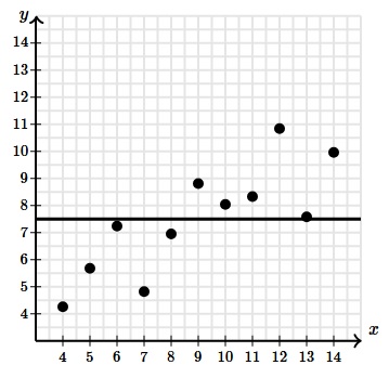
If we’d plot a line on the mean of y values, we’d see that the line doesn’t seem to fit the data well. One way to measure the fit of the line is to calculate the sum of the squared residuals. This gives us an overall sense of how much prediction error a given model has.

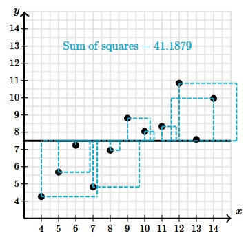
So without least-squares regression, our sum of squares is 41.1879.

Would using least-squares regression reduce the amount of prediction error? If so, by how much?

Predicting with regression

Here’s the same data with the corresponding least-squares regression line and summary statistics.

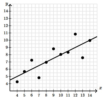
Equation: ŷ = 0.5x + 3
r = 0.816

This line seems to fit the data pretty well, but to measure how much better it fits, we can look again at the sum of the squared residuals.

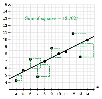
Using least-squares regression reduced the sum of the squared residuals from 41.1879 to 13.7627. So using least-squares regression eliminated a considerable amount of prediction error but how much?

R-squared measures how much prediction error we eliminated.

We can represent this reduction as a percentage of the original amount of prediction error.

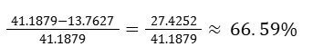
So the coefficient of determination, r² = 0.6659.

R-squared tells us what percent of the prediction error in the y variable is eliminated when we use least-squares regression on the x variable.

Another formal definition says that r-squared tells us what percent of the variability in the y variable is accounted for by the regression on the x variable.

It seems pretty remarkable that simply squaring r gives us this measurement. (However proving this relationship between r and r² is pretty complex, and is beyond the scope of an introductory statistics course.)

R-squared or coefficient of determination

In linear regression, r-squared (also called the coefficient of determination) is the proportion of variation in the response variable that is explained by the explanatory variable in the model.

Using the formula y=mx+b, we can write the total squared error of a line as:

SE_line = (y₁-(mx₁+b))² + (y₂-(mx₂+b))² + . . . + (y_n-(mx_n+b))²

If we want to come up with a more meaningful estimate of how good the (above) line is fitting the data points that we have, we can ask ourselves: How much (what percentage) of the total variation in y is described by the variation in x?

When we think about the total variation in y*, hence the squared distance from some central tendency, the best central measure we can have of y is the arithmetic mean.
(* also true for variance, that is the mean variation in y)

So total variation in y is going to be:

SE_ȳ = (y₁ – ȳ)² + (y₂ – ȳ)² + . . . + (y_n – ȳ)²

(if we divide the above by n, we’re going to get the variance of y, which is kind of the average squared distance)

SE_ȳ is referring to the squared error from the mean of y (aka total variation in y).

How much of the total variation is NOT described by the regression line?

That’s the total squared error of the line that we wrote above as the SE line.

So SE_line / SE_ȳ tells us what percentage of the variation is NOT described by the variation in x, or by the regression line.

What percentage of the total variation in y is described by the variation in x going to be:

That is also called the coefficient of determination or r².

If SE_line is small, then the line is a good fit, hence r-squared is close to 1.

If SE_line is large, then r-squared is close to 0.

Standard deviation of residuals or Root-mean-square error (RMSD)

Calculating the standard deviation of residuals (or root-mean-square error or root-mean-square deviation, RMSD) to measure disagreement between a linear regression model and a set of data.

As a reminder, the i’th residual is going to be:

r_i = y_i – ŷ

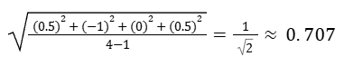
After we calculate all residuals, we can calculate the standard deviation of the residuals.

Let’s get back to our simple dataset with the data points (x, y):

(1, 1)
(2, 2)
(2, 3)
(3, 6)

The mean of x and y and their standard deviation were:

x̄ = 2
s_x = 0.816

ȳ = 3
s_y = 2.160

Our residuals would be:

r₁ = 1-0.5 = 0.5
r₂ = 2-3 = -1
r₃ = 3-3 = 0
r₄ = 6-5.5 = 0.5

So the standard deviation of the residuals is then:

(We can even draw lines, one SD above and one below the regression line.)

Because we are squaring the residuals, the outliers (things that are far from the line) are going to have a disproportionate impact here. If we didn’t want to have that behavior we could have done something like finding the mean of the absolute residuals, that actually in some ways would have been the simple one. But this is a standard way of people trying to figure out how much a model disagrees with the actual data.

So we can imagine, the lower this number (standard deviation of the residuals) is the better the fit of the model.

Interpreting computer regression data

Interpreting slope and y-intercept of regression line:

When we say the line (to model the data) has a slope of 22:

It means that the model predicts that the y-value (dependent) will increase 22 for each additional x value (independent).

When the line’s y-intercept is 42:

The model indicates that when the value of x is zero, the value of y would be 42.

Interpreting our estimate:

A “hat” on y is used to signify that this is an estimate. This estimate may be viewed as an average.

Let’s say we have the equation (ŷ = 41 + 0.59x) that predicts that possums with a total length of 80 cm will have an average head length of 88.2 mm. Absent further information about an 80 cm possum, the prediction for head length that uses the average is a reasonable estimate.

Interpreting regression analysis:

Let’s imagine we randomly select 20 students and record their caffeine intake (mg) and the number of hours spent studying. Assume that we have the following computer output from a least-squares regression analysis.

Predictor	Coef	SE Coef	T	P
Constant	2.544	0.134	18.955	0.000
Caffeine (mg)	0.164	0.057	2.862	0.005

S = 1.532 R-Sq = 60.032% R-Sq(adj) = 58.621%

y = hours studying
x = caffeine consumed

Our regression line would have the form: ŷ = mx + b

The coefficient on a constant is the constant. So our equation for the regression line is:
ŷ = 0.164x + 2.544

The other parts of the table (SE Coef, T and P) are useful for inferential statistics.

In the case above, r going to be:
r = √0.60032

We can tell that our r is positive by looking at the slope, that is also positive (0.164).

We don’t have to worry about the adjusted R-squared too much, when we’re thinking about just bivariate data. If we started to have more variables that tried to explain the hours studying, then we would care about adjusted R squared.

S is the standard deviation of the residuals. It is a measure of how well the regression line fits the data. It’s a measure of typical error.

Disclaimer: Like most of my posts, this content is intended solely for educational purposes and was created primarily for my personal reference. At times, I may rephrase original texts, and in some cases, I include materials such as graphs, equations, and datasets directly from their original sources.

I typically reference a variety of sources and update my posts whenever new or related information becomes available. For this particular post, the primary sources were Khan Academy’s Statistics and Probability series and OpenIntro Statistics by David Diez, Christopher Barr, & Mine Çetinkaya-Rundel.