Calculating conditional probability
Let’s assume we have the following probabilities.
- Eating simit for breakfast: P(A) = 0.6
- Eating doner for lunch: P(B) = 0.5
- (conditional probability of)*
eating simit for breakfast, given that eating doner for lunch: P(A|B) = 0.7
Based on these, what is the conditional probability that eating doner for lunch, given that eating simit for breakfast, P(B|A) = ?
We can tell these two events are dependent, since P(A|B) is different from P(A).
We also can write the following:
P(A and B) = P(A|B) * P (B) = P(B|A) * P(A)
0.7 * 0.5 = P(B|A) * 0.6
So P(B|A) would be 0.58333, ~0.58
* Math questions sometimes can be confusing in terms of wording. We may ask “why are we eating a simit for breakfast GIVEN we are eating a doner for lunch. Wouldn’t we eat lunch after breakfast?”
A better way to approach this could be: Suppose we eat doner for lunch that day, what’s the probability that we would have had a simit for breakfast that same day?
Conditional probability explained visually
Scenario 1: Unfair coin with equally likely events
Bob has two coins, one fair (H and T), another unfair (H and H).
He picks one at random, flips it and tells the result: Heads!
What’s the probability that he flipped the fair coin?
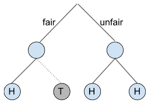
For this we can draw a tree:
First, our tree grows with two branches (fair and unfair).
The next event, he flips the coin.
Our tree grows again:
If he had a fair coin, it could result in H and T.
If he had an unfair coin, it could result in H and H.

Whenever we gain evidence (like announcing the result as Heads), we must trim our tree.
We cut any branch leading to Tails, because we know tails did not occur.
So, P(fair|H) = 1/3
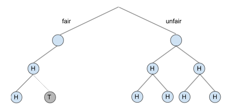
What happens if he flips again (the same coin) and reports again Heads?
After each event our tree grows.

Since he reported it’s Heads, we cut any branches leading to tails.
So, P(fair|HH) = 1/5
Our confidence in the fair coin is dropping as more Heads occur, though it will never reach zero.
No matter how many flips occur, we can never be 100% certain the coin is un/fair.
All conditional probability questions, P(A|B), can be solved by growing trees.
Scenario 2: Unfair coin without equally likely events
Let’s study another scenario: Bob has 3 coins, 2 fair and 1 biased, which is weighted to land Heads two thirds of the time and tails one third.
He picks one at random, flips it and tells the result: Heads!
What’s the probability that he chose a biased coin?
Again we start with growing our tree:

But we need to make sure that our tree is balanced, meaning an equal amount of leaves should grow out of each branch. To do this, we simply scale up the number of branches to the least common multiple. For 2 and 3, this is 6.

Since he announced the result as Heads, this new evidence allows us to trim all branches leading to tails.
So, P(biased|H) = 4/10
It’s also possible to answer conditional probability questions by Bayes’ Theorem.

P(A|B) = P(B|A) * P(A) / P(B)
Alper’s Notes
We can think of this also in two other ways:
First, as a simple equation as we saw before. That is:
P(A and B) = P(A|B) * P (B) = P(B|A) * P(A)
Or, second, as I prefer, we can reason it step-by-step:
0. We have a coin that says Heads and we are looking after the probability of it being a biased one.
1. Let’s start with having a biased coin in the first place.
→ It’s 1/3 of all coins.
2. Then we need to check having Heads within* a biased coin.
→ That’s 2/3.
3. We need to multiply these two, since we are checking both events happening together.
→ 1/3 · 2/3 = 2/9
4. Now we need to know how many of all outcomes were Heads. (Remember for 2 fair coin, it’s HT and for 1 unfair coin it’s HHT)
→ 1/3 · 1/2 + 1/3 · 1/2 + 1/3 · 2/3 = 10/18 = 5/9
5. Finally, we need the proportion of our target (getting a biased coin given a Head) among the focused subset (all possible Heads in the population).
→ (2/9) / (5/9) = 2/5 = 0.4 = 40%
* This shouldn’t be mixed with the term ‘given’, here I am thinking visually as all these steps in fact are subsets of a population (whole possible outcomes).
Scenario 3: Drug test with FP and FN rates
A company screens job applicants for illegal drug use at a certain stage in their hiring process. The specific test they use has a false positive rate of 2% and a false negative rate of 1%. Suppose that 5% of all their applicants are actually using illegal drugs, and we randomly select an applicant.
Given that applicant tests positive, what is the probability that they are actually on drugs?
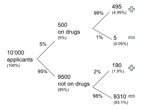
We can draw our tree again, let’s say we have 10’000 applicants.

We have 495+190 tested positive, and among all of them 495 were actually on drugs.
So, 495 / (495+190) = ~72%
We could also get this result just by using the percentages as 4.95% / (4.95% + 1.9%).
That’s interesting! When we look at the FP and FN rates, they seem quite low. But now, when we actually did the calculation, the probability that someone is actually on drugs is, -say- high, but not that high. We can’t tell that person is definitely taking the drugs.
This is saying, of the people that test positive, 72% are actually on the drugs. Or another way to say is, if someone tests positive using this test, there’s a 28% chance that they are not taking drugs.
Scenario 4: Conditional probability and independence
We have a table below, showing the weather conditions and whether the train runs on time or not. For these days, are the events ‘delayed’ and ‘snowy’ independent?
| On time | Delayed | Total | |
| Sunny | 167 | 3 | 170 |
| Cloudy | 115 | 5 | 120 |
| Rainy | 40 | 15 | 55 |
| Snowy | 8 | 12 | 20 |
| Total | 330 | 35 | 365 |
Remember, the more experiments we’re able to take, the more likely it is to approximate the true theoretical probability. But there is always a chance that they might be different or even quite different. Let’s use this data above to try to calculate the experimental probability.
The key questions here are, what is P(delayed) and P(delayed | snowy)?
If we knew the theoretical probabilities and if they were exactly the same, then being delayed or being snowy would be independent. But we don’t know the theoretical probabilities, we’re just going to calculate the experimental probabilities. And we do have a good number of experiments here (those in the table above).
P(delayed) = 35 / 365, that is < 0.1
P(delayed | snowy) = 12 / 20 = 0.6
From the experimental data, it seems that a much higher proportion of our snowy days are delayed than just in general days. Because the experimental probability of being delayed given snowy is so much higher than the experimental probability of just being delayed, we would make the statement that these are not independent.
Let’s write this in math notation:
If P(A | B) = P(A) we can say A and B are independent.
Or P(B | A) = P(B) would mean that they are independent.
Or P(A and B) = P(A) * P(B) also means that they are independent.
What if the probabilities are close?
When we check for independence in real world data sets, it’s rare to get perfectly equal probabilities. Just about all real events that don’t involve games of chance are dependent to some degree.
In practice, we often assume that events are independent and test that assumption on sample data. If the probabilities are significantly different, then we conclude the events are not independent.
Finally, we need to be careful not to make conclusions about cause and effect unless the data came from a well-designed experiment.
Disclaimer: Like most of my posts, this content is intended solely for educational purposes and was created primarily for my personal reference. At times, I may rephrase original texts, and in some cases, I include materials such as graphs, equations, and datasets directly from their original sources.
I typically reference a variety of sources and update my posts whenever new or related information becomes available. For this particular post, the primary source was Khan Academy’s Statistics and Probability series.
