Here we’ll quickly demonstrate a logistic regression in Python by using a dataset that comes from a study about motion detection in older adults. We’ll work with a subset of this data.
There are two variables in the dataset. The first variable measures acceleration in the vertical direction. The second variable indicates whether a person is lying down. We want to use logistic regression to predict whether the person is lying down or not.
Begin by importing the relevant packages and data.
Exploratory data analysis
# Import pandas and seaborn packages
import pandas as pd
import seaborn as sns
# Load dataset
activity = pd.read_csv("activity.csv")
# Examine the dataset
activity.head()| Acc (vertical) | LyingDown | |
|---|---|---|
| 0 | 96.229 | 0 |
| 1 | 84.746 | 0 |
| 2 | 82.449 | 0 |
| 3 | 106.560 | 0 |
| 4 | 80.152 | 0 |
# Get summary statistics about the dataset
activity.describe()| Acc (vertical) | LyingDown | |
|---|---|---|
| count | 494.000000 | 494.000000 |
| mean | 45.512363 | 0.516194 |
| std | 44.799360 | 0.500244 |
| min | -48.459000 | 0.000000 |
| 25% | 0.918650 | 0.000000 |
| 50% | 41.109500 | 1.000000 |
| 75% | 89.339000 | 1.000000 |
| max | 112.310000 | 1.000000 |
Construct binomial logistic regression model
# Load in sci-kit learn functions for constructing logistic regression
from sklearn.model_selection import train_test_split
from sklearn.linear_model import LogisticRegression
# Save X and y data into variables
X = activity[["Acc (vertical)"]]
y = activity[["LyingDown"]]# Split dataset into training and holdout datasets
X_train, X_test, y_train, y_test = train_test_split(X,y, test_size=0.3, random_state=42)clf = LogisticRegression().fit(X_train,y_train)Get coefficients and visualize model
# Print the coefficient
clf.coef_
array([[-0.1177466]])
# Print the intercept
clf.intercept_
array([6.10177895])
So, based on what we’ve found, our model has an intercept or β0 of 6.10 and a β1 of -0.12. Now we can plot our model and data with a 95% confidence band using the regplot() function from the seaborn package. We need to set the argument logistic=True so that the function knows we are plotting a logistic regression model, not a linear regression model.
# Plot the logistic regression and its confidence band
sns.regplot(x="Acc (vertical)", y="LyingDown", data=activity, logistic=True)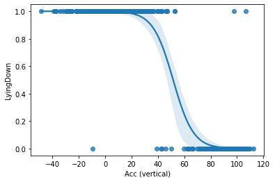
Evaluate the Model
Construct logistic regression model
We’ve already built our regression model and now we can save our model’s predictions by inputting the holdout sample, X_test into the model’s .predict() function.
# Save predictions
y_pred = clf.predict(X_test)
We can also print out the predicted labels if we wanted to see the predictions.
# Print out the predicted labels
clf.predict(X_test)
array([0, 1, 0, 0, 1, 0, 0, 1, 1, 0, 1, 0, 0, 1, 1, 0, 0, 0, 1, 1, 0, 1,
1, 0, 1, 0, 1, 1, 0, 1, 0, 0, 1, 0, 1, 0, 1, 1, 1, 1, 0, 1, 0, 1,
0, 0, 0, 0, 0, 0, 1, 0, 0, 1, 0, 1, 0, 1, 0, 1, 0, 0, 0, 1, 0, 0,
1, 1, 0, 0, 1, 0, 0, 0, 0, 0, 1, 1, 0, 0, 0, 1, 1, 0, 1, 0, 1, 1,
1, 0, 1, 0, 1, 1, 1, 1, 1, 0, 1, 1, 0, 0, 1, 1, 1, 1, 1, 1, 1, 0,
0, 0, 1, 0, 1, 1, 0, 1, 1, 1, 1, 1, 1, 0, 1, 1, 0, 1, 1, 0, 1, 0,
0, 1, 0, 0, 1, 1, 0, 1, 0, 1, 0, 0, 1, 0, 1, 1, 1])
As we know already, the model actually calculates a probability that given a particular value of X, the person is lying down. We can also print out the predicted probabilities with the following line of code.
# Print out the predicted probabilities
clf.predict_proba(X_test)[::,-1]
array([2.31693308e-02, 9.97511568e-01, 1.04282071e-02, 1.05672351e-03,
9.99781257e-01, 1.04282071e-02, 4.66017106e-03, 9.95733864e-01,
9.72343955e-01, 2.31693308e-02, 9.97825589e-01, 1.36212174e-02,
3.43616982e-02, 9.95733864e-01, 9.98892860e-01, 5.75929752e-02,
4.77298577e-01, 6.09795092e-03, 9.98732777e-01, 9.92695617e-01,
3.91403776e-02, 9.31712676e-01, 9.64063419e-01, 1.55638073e-02,
9.83708329e-01, 1.19195424e-02, 7.55107906e-01, 8.74057100e-01,
3.43616982e-02, 9.91646273e-01, 1.77763901e-02, 1.19195424e-02,
9.97152314e-01, 2.64340977e-02, 9.98892860e-01, 1.19195424e-02,
9.31712676e-01, 9.95119247e-01, 9.00935568e-01, 9.22594161e-01,
8.39846087e-02, 9.99624389e-01, 1.19195424e-02, 8.01629006e-01,
5.33106480e-03, 1.36212174e-02, 3.01447030e-02, 3.55976011e-03,
4.07288328e-03, 1.19195424e-02, 9.98892860e-01, 6.53836704e-02,
4.07288328e-03, 9.98892860e-01, 9.12067619e-03, 9.53422359e-01,
1.20976784e-03, 9.89081439e-01, 6.53836704e-02, 9.99950563e-01,
3.55976011e-03, 4.66017106e-03, 9.49855175e-02, 9.99713340e-01,
6.09795092e-03, 2.71879989e-03, 9.98732777e-01, 9.92695617e-01,
2.02970330e-02, 4.66017106e-03, 9.92695617e-01, 4.66017106e-03,
3.55976011e-03, 8.06224240e-04, 1.77763901e-02, 5.75929752e-02,
9.83708329e-01, 9.98732777e-01, 5.75929752e-02, 2.12858682e-01,
1.55638073e-02, 9.78756075e-01, 9.98339943e-01, 1.07258677e-01,
9.53422359e-01, 6.97519741e-03, 9.97511568e-01, 9.99261761e-01,
9.99671864e-01, 1.04282071e-02, 9.96271374e-01, 1.55638073e-02,
9.98339943e-01, 9.98892860e-01, 9.87520863e-01, 9.31712676e-01,
9.47037987e-01, 2.64340977e-02, 7.55107906e-01, 9.99569998e-01,
4.66017106e-03, 3.91403776e-02, 8.22251990e-01, 9.99154973e-01,
9.39833736e-01, 9.39833736e-01, 9.98549580e-01, 9.85738795e-01,
9.93613325e-01, 9.12067619e-03, 6.97519741e-03, 1.19195424e-02,
9.99713340e-01, 6.97519741e-03, 9.99671864e-01, 9.95733864e-01,
4.45529655e-02, 9.59075003e-01, 9.99935211e-01, 9.99569998e-01,
8.01629006e-01, 9.81394227e-01, 5.44778650e-01, 1.36212174e-02,
9.97825589e-01, 9.93613325e-01, 1.36212174e-02, 9.99781257e-01,
9.99154973e-01, 3.43616982e-02, 9.68463782e-01, 6.97519741e-03,
1.55638073e-02, 9.75755881e-01, 2.02970330e-02, 5.75929752e-02,
9.92695617e-01, 9.47037987e-01, 1.04282071e-02, 9.99355101e-01,
1.36212174e-02, 9.87520863e-01, 2.02970330e-02, 7.41453115e-02,
9.85738795e-01, 2.37530617e-03, 9.78756075e-01, 9.98732777e-01,
9.97511568e-01])
Create confusion matrix
To create a confusion matrix, we’ll use the confusion_matrix() function from the metrics module of scikit-learn. To use the function, we’ll need to input the following:
- Actual labels of the holdout sample, stored as
y_test - Predicted labels of the holdout sample, stored as
y_pred - The names of the labels, which we can access using
clf.classes_
Note: If there were more classes, we would have more numbers or labels in clf.classes_. Since this is a binomial logistic regression, there are only two labels, 0 and 1.
# Import the metrics module from scikit-learn
import sklearn.metrics as metrics
# Calculate the values for each quadrant in the confusion matrix
cm = metrics.confusion_matrix(y_test, y_pred, labels = clf.classes_)
# Create the confusion matrix as a visualization
disp = metrics.ConfusionMatrixDisplay(confusion_matrix = cm, display_labels = clf.classes_)# Display the confusion matrix
disp.plot()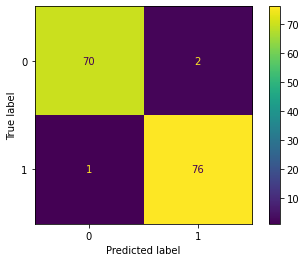
We can define the confusion matrix in our given context as:
- True negatives: The number of people (here 70) that were not lying down that the model accurately predicted as not lying down.
- False negatives: The number of people (here 1) that were lying down that the model inaccurately predicted as not lying down.
- False positives: The number of people (here 2) that were not lying down that the model inaccurately predicted as lying down.
- True positives: The number of people (here 76) that were lying down that the model accurately predicted as lying down.
Disclaimer: Like most of my posts, this content is intended solely for educational purposes and was created primarily for my personal reference. At times, I may rephrase original texts, and in some cases, I include materials such as graphs, equations, and datasets directly from their original sources.
I typically reference a variety of sources and update my posts whenever new or related information becomes available. For this particular post, the primary source was Google Advanced Data Analytics Professional Certificate.