At the core of all of our regression analysis and statistics is storytelling. We want to understand how the different variables are related, although regression and ANOVA can help answer similar questions, one or the other might be more useful in specific cases.
A regression analysis will help provide a holistic picture of if and by how much a number of different variables impact an outcome variable.
On the other hand ANOVA helps unpack pairwise comparisons (among subsets of those variables), to better understand the nuances among the elements that fuel the regression analysis. ANOVA can work like a magnifying glass zooming in on specific parts of the regression story.
One-way ANOVA
# Import pandas and seaborn packages
import pandas as pd
import seaborn as sns
# Load in diamonds data set from seaborn package
diamonds = sns.load_dataset("diamonds", cache=False)
# Examine first 5 rows of data set
diamonds.head()| carat | cut | color | clarity | depth | table | price | x | y | z | |
|---|---|---|---|---|---|---|---|---|---|---|
| 0 | 0.23 | Ideal | E | SI2 | 61.5 | 55.0 | 326 | 3.95 | 3.98 | 2.43 |
| 1 | 0.21 | Premium | E | SI1 | 59.8 | 61.0 | 326 | 3.89 | 3.84 | 2.31 |
| 2 | 0.23 | Good | E | VS1 | 56.9 | 65.0 | 327 | 4.05 | 4.07 | 2.31 |
| 3 | 0.29 | Premium | I | VS2 | 62.4 | 58.0 | 334 | 4.20 | 4.23 | 2.63 |
| 4 | 0.31 | Good | J | SI2 | 63.3 | 58.0 | 335 | 4.34 | 4.35 | 2.75 |
Data cleaning
Here, our main focus is on one-way and two-way ANOVA. This means that our dataset needs a continuous variable, and up to two categorical variables.
Note: In the workplace, we will always start with a business problem and the data, and then determine the best models or tests to run on the data. We will never work in the reverse. For educational purposes, here we’ll focus only on ANOVA.
# Check how many diamonds are each color grade
diamonds["color"].value_counts()
G 11292 E 9797 F 9542 H 8304 D 6775 I 5422 J 2808 Name: color, dtype: int64
# Subset for colorless diamonds
colorless = diamonds[diamonds["color"].isin(["E","F","H","D","I"])]

# Select only color and price columns, and reset index
colorless = colorless[["color","price"]].reset_index(drop=True)
Note: We took a subset of colorless and near colorless diamonds. We excluded G color grade diamonds as there were many more of them, and we excluded J color grade diamonds as there were significantly fewer of them. In a workplace setting, we would typically go through a more thoughtful process of subsetting. Again, the goal of this work is focusing on ANOVA, not data cleaning or variable selection.
# Remove dropped categories of diamond color
colorless.color = colorless.color.cat.remove_categories(["G","J"])

# Check that the dropped categories have been removed
colorless["color"].values
['E', 'E', 'E', 'I', 'I', ..., 'D', 'D', 'D', 'H', 'D'] Length: 39840 Categories (5, object): ['D', 'E', 'F', 'H', 'I']
# Import math package
import math

# Take the logarithm of the price, and insert it as the third column
colorless.insert(2, "log_price", [math.log(price) for price in colorless["price"]])
The first argument in the insert() function allows us to specify the location of the new column with a column number. But the argument starts counting at 0. So if we put in 0, that is the first column; if we enter 1, that is the second column, and so on. Since we specified 2, the new log_price column will be the third column.
# Drop rows with missing values
colorless.dropna(inplace=True)

# Reset index
colorless.reset_index(inplace=True, drop=True)
Next, we use the dropna() function to drop the rows with missing values. Setting the inplace argument to True means that we do not have to save the dataframe as a new variable. Then, we’ll reset the index using the reset_index() function to reset the index column to account for the rows we just dropped. The inplace argument works the same as it did for the dropna() function, and the drop argument prevents us from creating a new column with the old index numbers preserved.
# Examine first 5 rows of cleaned data set
colorless.head()| color | price | log_price | |
|---|---|---|---|
| 0 | E | 326 | 5.786897 |
| 1 | E | 326 | 5.786897 |
| 2 | E | 327 | 5.789960 |
| 3 | I | 334 | 5.811141 |
| 4 | I | 336 | 5.817111 |
# Save to diamonds.csv
colorless.to_csv('diamonds.csv',index=False,header=list(colorless.columns))
The code creates a new .csv file of the colorless dataframe, and names it diamonds.csv. The index argument tells the function whether or not we want to save the index column as a column in the .csv file. Additionally, the header argument tells the function what the names of the columns should be.
Perform One-way ANOVA
To run one-way ANOVA, we first load in the data, and save it as a variable called diamonds, and then examine it using the head() function.
# Save diamonds.csv as a variable called diamonds
diamonds = pd.read_csv("diamonds.csv")

# Examine first 5 rows of diamonds data set
diamonds.head()| color | price | log_price | |
|---|---|---|---|
| 0 | E | 326 | 5.786897 |
| 1 | E | 326 | 5.786897 |
| 2 | E | 327 | 5.789960 |
| 3 | I | 334 | 5.811141 |
| 4 | I | 336 | 5.817111 |
Recall that one-way ANOVA helps us better understand the relationship between a categorical variable and a continuous variable. We’ll do some basic exploratory data analysis by creating a boxplot using the boxplot() function from the seaborn package.
# Create boxplot to show distribution of price by color grade
sns.boxplot(x = "color", y = "log_price", data = diamonds)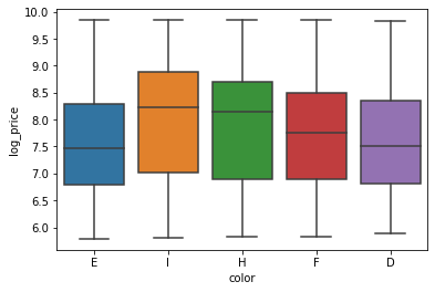
Based on the plot, we can observe that there is a lot of overlap in the distribution of log_price for each color of diamond. But we can’t tell yet if they are statistically significantly different.
In order to run ANOVA, we need to create a regression model. To do this, we’ll import the statsmodels.api package and the ols() function. Next, we’ll create a simple linear regression model where the X variable is color, which we will code as categorical using C(). Then, we’ll fit the model to the data, and generate model summary statistics.
# Import statsmodels and ols function
import statsmodels.api as sm
from statsmodels.formula.api import ols

# Construct simple linear regression model, and fit the model
model = ols(formula = "log_price ~ C(color)", data = diamonds).fit()

# Get summary statistics
model.summary()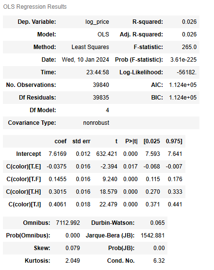
Warnings:
[1] Standard Errors assume that the covariance matrix of the errors is correctly specified.
Based on the model summary table, the color grades’ associated beta coefficients all have a p-value of less than 0.05 (check the P>|t| column). But we can’t be sure if there is a significant price difference between the various color grades. This is where one-way ANOVA comes in.
First, we have to state our null and alternative hypotheses:
Null Hypothesis
H0 : priceD = priceE = priceF = priceH = priceI
There is no difference in the price of diamonds based on color grade.
Alternative Hypothesis
H1 : Not priceD = priceE = priceF = priceH = priceI
There is a difference in the price of diamonds based on color grade.
# Run one-way ANOVA
sm.stats.anova_lm(model, typ = 2)| sum_sq | df | F | PR(>F) | |
|---|---|---|---|---|
| C(color) | 1041.690290 | 4.0 | 264.987395 | 3.609774e-225 |
| Residual | 39148.779822 | 39835.0 | NaN | NaN |
sm.stats.anova_lm(model, typ = 1)| df | sum_sq | mean_sq | F | PR(>F) | |
|---|---|---|---|---|---|
| C(color) | 4.0 | 1041.690290 | 260.422572 | 264.987395 | 3.609774e-225 |
| Residual | 39835.0 | 39148.779822 | 0.982773 | NaN | NaN |
sm.stats.anova_lm(model, typ = 3)| sum_sq | df | F | PR(>F) | |
|---|---|---|---|---|
| Intercept | 393066.804852 | 1.0 | 399956.684283 | 0.000000e+00 |
| C(color) | 1041.690290 | 4.0 | 264.987395 | 3.609774e-225 |
| Residual | 39148.779822 | 39835.0 | NaN | NaN |
We use the anova_lm() function from the statsmodels.stats package. As noted previously, the function requires a fitted regression model, and for us to specify the type of ANOVA: 1, 2, or 3. Since the p-value (column PR(>F)) is very small, we can reject the null hypothesis that the mean of the price is the same for all diamond color grades.
Technical note: The type of an ANOVA and the number of ways of an ANOVA are two distinct concepts: “type” (typ in statsmodels.stats.anova.anova_lm()) refers to how the sums of squares (these quantities are the building blocks for ANOVA) are calculated, while “K-way” means that there are K categorical factors in the analysis.
Two-Way ANOVA
Data cleaning
Now, we will prepare a second dataset so we can perform a two-way ANOVA, which requires two categorical variables. We will start with the same diamonds dataset from the seaborn package.
# Import diamonds data set from seaborn package
diamonds = sns.load_dataset("diamonds", cache=False)
# Examine first 5 rows of data set
diamonds.head()| carat | cut | color | clarity | depth | table | price | x | y | z | |
|---|---|---|---|---|---|---|---|---|---|---|
| 0 | 0.23 | Ideal | E | SI2 | 61.5 | 55.0 | 326 | 3.95 | 3.98 | 2.43 |
| 1 | 0.21 | Premium | E | SI1 | 59.8 | 61.0 | 326 | 3.89 | 3.84 | 2.31 |
| 2 | 0.23 | Good | E | VS1 | 56.9 | 65.0 | 327 | 4.05 | 4.07 | 2.31 |
| 3 | 0.29 | Premium | I | VS2 | 62.4 | 58.0 | 334 | 4.20 | 4.23 | 2.63 |
| 4 | 0.31 | Good | J | SI2 | 63.3 | 58.0 | 335 | 4.34 | 4.35 | 2.75 |
Below, we go through a very similar process as above.
- We start by selecting the columns of interest:
color,cut, andprice. Then, we subset only for certain color grades, and remove the dropped colors from the list of categories using theremove_categories()function. - Next, we subset for specific diamond cuts:
Ideal,Premium, andVery Good, and remove the dropped cuts from the list of categories. - Next, we remove rows with missing data, and reset the index.
- Lastly, we add in a column for the logarithm of the price.
# Subset for color, cut, price columns
diamonds2 = diamonds[["color","cut","price"]]

# Only include colorless diamonds
diamonds2 = diamonds2[diamonds2["color"].isin(["E","F","H","D","I"])]

# Drop removed colors, G and J
diamonds2.color = diamonds2.color.cat.remove_categories(["G","J"])

# Only include ideal, premium, and very good diamonds
diamonds2 = diamonds2[diamonds2["cut"].isin(["Ideal","Premium","Very Good"])]

# Drop removed cuts
diamonds2.cut = diamonds2.cut.cat.remove_categories(["Good","Fair"])

# Drop NaNs
diamonds2.dropna(inplace = True)

# Reset index
diamonds2.reset_index(inplace = True, drop = True)

# Add column for logarithm of price
diamonds2.insert(3,"log_price",[math.log(price) for price in diamonds2["price"]])
# Examine the data set
diamonds2.head()| color | cut | price | log_price | |
|---|---|---|---|---|
| 0 | E | Ideal | 326 | 5.786897 |
| 1 | E | Premium | 326 | 5.786897 |
| 2 | I | Premium | 334 | 5.811141 |
| 3 | I | Very Good | 336 | 5.817111 |
| 4 | H | Very Good | 337 | 5.820083 |
We save the dataset as a .csv file again using the to_csv() function, just as above.
# Save as diamonds2.csv
diamonds2.to_csv('diamonds2.csv',index=False,header=list(diamonds2.columns))
Perform Two-Way ANOVA
# Load the data set
diamonds2 = pd.read_csv("diamonds2.csv")
# Examine the first 5 rows of the data set
diamonds2.head()| color | cut | price | log_price | |
|---|---|---|---|---|
| 0 | E | Ideal | 326 | 5.786897 |
| 1 | E | Premium | 326 | 5.786897 |
| 2 | I | Premium | 334 | 5.811141 |
| 3 | I | Very Good | 336 | 5.817111 |
| 4 | H | Very Good | 337 | 5.820083 |
Then we’ll create a multiple linear regression model using the ols() function, fit the model to the data, and get the summary statistics.
Note: This regression model includes two categorical X variables: color and cut, and a variable to account for the interaction between color and cut. The interaction is denoted using the : symbol.
# Construct a multiple linear regression with an interaction term between color and cut
model2 = ols(formula = "log_price ~ C(color) + C(cut) + C(color):C(cut)", data = diamonds2).fit()

# Get summary statistics
model2.summary()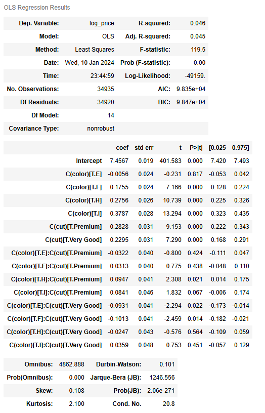
Warnings:
[1] Standard Errors assume that the covariance matrix of the errors is correctly specified.
Based on the model summary table, many of the color grades’ and cuts’ associated beta coefficients have a p-value of less than 0.05 (check the P>|t| column). Additionally, some of the interactions also seem statistically significant. We’ll use a two-way ANOVA to examine further the relationships between price and the two categories of color grade and cut.
First, we have to state our three pairs of null and alternative hypotheses:
Null Hypothesis (Color)
H0 : priceD = priceE = priceF = priceH = priceI
There is no difference in the price of diamonds based on color.
Alternative Hypothesis (Color)
H1 : Not priceD = priceE = priceF = priceH = priceI
There is a difference in the price of diamonds based on color.
Null Hypothesis (Cut)
H0 : priceIdeal = pricePremium = priceVery Good
There is no difference in the price of diamonds based on cut.
Alternative Hypothesis (Cut)
H1 : Not priceIdeal = pricePremium = priceVery Good
There is a difference in the price of diamonds based on cut.
Null Hypothesis (Interaction)
H0 : The effect of color on diamond price is independent of the cut, and vice versa.
Alternative Hypothesis (Interaction)
H1 : There is an interaction effect between color and cut on diamond price.
The syntax for a two-way ANOVA is the same as for a one-way ANOVA. We will continue to use the anova_lm() function from statsmodels.stats.
# Run two-way ANOVA
sm.stats.anova_lm(model2, typ = 2)| sum_sq | df | F | PR(>F) | |
|---|---|---|---|---|
| C(color) | 926.361461 | 4.0 | 237.014783 | 3.481145e-201 |
| C(cut) | 630.641441 | 2.0 | 322.706309 | 1.348511e-139 |
| C(color):C(cut) | 27.478611 | 8.0 | 3.515279 | 4.531734e-04 |
| Residual | 34120.806577 | 34920.0 | NaN | NaN |
sm.stats.anova_lm(model2, typ = 1)| df | sum_sq | mean_sq | F | PR(>F) | |
|---|---|---|---|---|---|
| C(color) | 4.0 | 977.195814 | 244.298954 | 250.021037 | 3.747388e-212 |
| C(cut) | 2.0 | 630.641441 | 315.320721 | 322.706309 | 1.348511e-139 |
| C(color):C(cut) | 8.0 | 27.478611 | 3.434826 | 3.515279 | 4.531734e-04 |
| Residual | 34920.0 | 34120.806577 | 0.977114 | NaN | NaN |
sm.stats.anova_lm(model2, typ = 3)| sum_sq | df | F | PR(>F) | |
|---|---|---|---|---|
| Intercept | 157578.043681 | 1.0 | 161268.910012 | 0.000000e+00 |
| C(color) | 319.145817 | 4.0 | 81.655250 | 4.134649e-69 |
| C(cut) | 100.144107 | 2.0 | 51.244864 | 5.987341e-23 |
| C(color):C(cut) | 27.478611 | 8.0 | 3.515279 | 4.531734e-04 |
| Residual | 34120.806577 | 34920.0 | NaN | NaN |
Since all of the p-values (column PR(>F)) are very small, we can reject all three null hypotheses.
Disclaimer: Like most of my posts, this content is intended solely for educational purposes and was created primarily for my personal reference. At times, I may rephrase original texts, and in some cases, I include materials such as graphs, equations, and datasets directly from their original sources.
I typically reference a variety of sources and update my posts whenever new or related information becomes available. For this particular post, the primary source was Google Advanced Data Analytics Professional Certificate.