Introduction
ANOVA, analysis of variance is a group of statistical techniques that test the difference of means among three or more groups. It’s a powerful tool for determining whether population means are different across groups and for answering a wide range of business questions.
Here we’ll assume that we are a data professional working with historical marketing promotion data. We will use the data to run a one-way ANOVA and a post hoc ANOVA test. Then, we will communicate our results to stakeholders.
In our dataset, each row corresponds to an independent marketing promotion, where our business uses TV, social media, radio, and influencer promotions to increase sales. We have previously provided insights about how different promotion types affect sales; now stakeholders want to know if sales are significantly different among various TV and influencer promotion types.
To address this request, a one-way ANOVA test will enable us to determine if there is a statistically significant difference in sales among groups. This includes:
- Using plots and descriptive statistics to select a categorical independent variable
- Creating and fitting a linear regression model with the selected categorical independent variable
- Checking model assumptions
- Performing and interpreting a one-way ANOVA test
- Comparing pairs of groups using an ANOVA post hoc test
- Interpreting model outputs and communicating the results to nontechnical stakeholders
Step 1: Imports
# Import libraries and packages.
import pandas as pd
import matplotlib.pyplot as plt
import seaborn as sns
import statsmodels.api as sm
from statsmodels.formula.api import ols
from statsmodels.stats.multicomp import pairwise_tukeyhsd
The variables in the dataset have been adjusted to suit the objectives of this work.
# Load the data.
data = pd.read_csv('marketing_sales_data.csv')

# Display the first five rows.
data.head()| TV | Radio | Social Media | Influencer | Sales | |
|---|---|---|---|---|---|
| 0 | Low | 1.218354 | 1.270444 | Micro | 90.054222 |
| 1 | Medium | 14.949791 | 0.274451 | Macro | 222.741668 |
| 2 | Low | 10.377258 | 0.061984 | Mega | 102.774790 |
| 3 | High | 26.469274 | 7.070945 | Micro | 328.239378 |
| 4 | High | 36.876302 | 7.618605 | Mega | 351.807328 |
The features in the data are:
- TV promotion budget (in Low, Medium, and High categories)
- Social media promotion budget (in millions of dollars)
- Radio promotion budget (in millions of dollars)
- Sales (in millions of dollars)
- Influencer size (in Mega, Macro, Nano, and Micro categories)
Step 2: Data exploration
Let’s check how Sales vary based on the TV promotion budget category.
# Create a boxplot with TV and Sales
sns.boxplot(x = "TV", y = "Sales", data = data)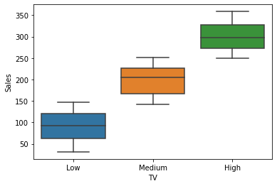
There is considerable variation in Sales across the TV groups. The significance of these differences can be tested with a one-way ANOVA.
Now, we’ll check how Sales vary based on the Influencer size category.
# Create a boxplot with Influencer and Sales
sns.boxplot(x = "Influencer", y = "Sales", data = data)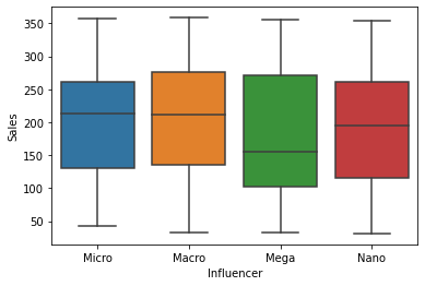
There is some variation in Sales across the Influencer groups, but it may not be significant.
Remove missing data
# Drop rows that contain missing data and update the DataFrame
data = data.dropna(axis=0)

# Confirm the data contain no missing values
data.isnull().sum(axis=0)
TV 0 Radio 0 Social Media 0 Influencer 0 Sales 0 dtype: int64
Step 3: Model building
# Define the OLS formula
ols_formula = 'Sales ~ C(TV)'

# Create an OLS model
OLS = ols(formula = ols_formula, data = data)

# Fit the model
model = OLS.fit()

# Save the results summary
model_results = model.summary()

# Display the model results
model_results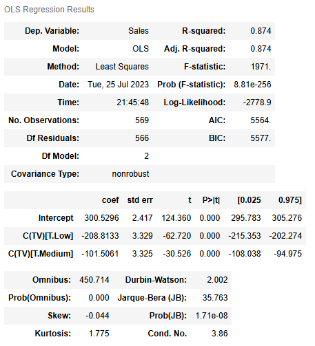
Warnings:
[1] Standard Errors assume that the covariance matrix of the errors is correctly specified.
TVwas selected as the preceding analysis showed a strong relationship between theTVpromotion budget and the averageSales.Influencerwas not selected because it did not show a strong relationship toSalesin the analysis.
Check model assumptions
Because your model does not have any continuous independent variables, the linearity assumption is not required.
The independent observation assumption states that each observation in the dataset is independent. As each marketing promotion (row) is independent from one another, the independence assumption is not violated.
Now lets check the normality assumption.
# Calculate the residuals
residuals = model.resid

# Create a 1x2 plot figure
fig, axes = plt.subplots(1, 2, figsize = (8,4))

# Create a histogram with the residuals
sns.histplot(residuals, ax=axes[0])
# Set the x label of the residual plot
axes[0].set_xlabel("Residual Value")
# Set the title of the residual plot
axes[0].set_title("Histogram of Residuals")

# Create a QQ plot of the residuals
sm.qqplot(residuals, line='s',ax = axes[1])
# Set the title of the QQ plot
axes[1].set_title("Normal QQ Plot")

# Use matplotlib's tight_layout() function to add space between plots for a cleaner appearance
plt.tight_layout()
# Show the plot
plt.show()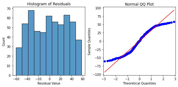
There is reasonable concern that the normality assumption is not met when TV is used as the independent variable predicting Sales. The normal q-q forms an ‘S’ that deviates off the red diagonal line, which is not desired behavior.
However, for the purpose of this work, we’ll continue assuming the normality assumption is met.
Now, let’s verify the constant variance (homoscedasticity) assumption is met or not.
# Create a scatter plot with the fitted values from the model and the residuals
fig = sns.scatterplot(x = model.fittedvalues, y = model.resid)

# Set the x axis label
fig.set_xlabel("Fitted Values")
# Set the y axis label
fig.set_ylabel("Residuals")
# Set the title
fig.set_title("Fitted Values v. Residuals")

# Add a line at y = 0 to visualize the variance of residuals above and below 0
fig.axhline(0)

# Show the plot
plt.show()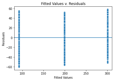
The variance where there are fitted values is similarly distributed, validating that the constant variance assumption is met.
Step 4: Results and evaluation
# Display the model results summary
model_results- Using
TVas the independent variable results in a linear regression model with R2=0.874. In other words, the model explains 87.4% of the variation inSales. This makes the model an effective predictor ofSales.
- The default
TVcategory for the model isHigh, because there are coefficients for the other twoTVcategories,MediumandLow. According to the model,Saleswith aMediumorLowTVcategory are lower on average thanSaleswith aHighTVcategory. For example, the model predicts that aLowTVpromotion would be 208.813 (in millions of dollars) lower inSaleson average than aHighTVpromotion.
- The p-value for all coefficients is 0.0000.000, meaning all coefficients are statistically significant at p=0.05. The 95% confidence intervals for each coefficient should be reported when presenting results to stakeholders. For instance, there is a 95% chance the interval [−215.353,−202.274] contains the true parameter of the slope of βTVLow, which is the estimated difference in promotion sales when a
LowTVpromotion is chosen instead of aHighTVpromotion.
- Given how accurate
TVwas as a predictor, the model could be improved with a more granular view of theTVpromotions, such as additional categories or the actualTVpromotion budgets. Further, additional variables, such as the location of the marketing campaign or the time of year, may increase model accuracy.
Perform a one-way ANOVA test
With the model fit, now we’ll run a one-way ANOVA test to determine whether there is a statistically significant difference in Sales among groups.
# Create an one-way ANOVA table for the fit model
sm.stats.anova_lm(model, typ=2)| sum_sq | df | F | PR(>F) | |
|---|---|---|---|---|
| C(TV) | 4.052692e+06 | 2.0 | 1971.455737 | 8.805550e-256 |
| Residual | 5.817589e+05 | 566.0 | NaN | NaN |
- The null hypothesis is that there is no difference in
Salesbased on theTVpromotion budget. - The alternative hypothesis is that there is a difference in
Salesbased on theTVpromotion budget.
- The F-test statistic is 1971.46 and the p-value is 8.81∗10−256 (i.e., very small). Because the p-value is less than 0.05, we would reject the null hypothesis that there is no difference in
Salesbased on theTVpromotion budget.
- The results of the one-way ANOVA test indicate that we can reject the null hypothesis in favor of the alternative hypothesis. There is a statistically significant difference in
SalesamongTVgroups.
Perform an ANOVA post hoc test
If we have significant results from the one-way ANOVA test, we can apply ANOVA post hoc tests such as the Tukey’s HSD post hoc test, to compare if there is a significant difference between each pair of categories for TV.
# Perform the Tukey's HSD post hoc test
tukey_oneway = pairwise_tukeyhsd(endog = data["Sales"], groups = data["TV"])

# Display the results
tukey_oneway.summary()| group1 | group2 | meandiff | p-adj | lower | upper | reject |
|---|---|---|---|---|---|---|
| High | Low | -208.8133 | 0.001 | -216.637 | -200.9896 | True |
| High | Medium | -101.5061 | 0.001 | -109.3204 | -93.6918 | True |
| Low | Medium | 107.3072 | 0.001 | 99.7063 | 114.908 | True |
- The first row, which compares the
HighandLowTVgroups, indicates that we can reject the null hypothesis that there is no significant difference between theSalesof these two groups. - We can also reject the null hypotheses for the two other pairwise comparisons that compare
HightoMediumandLowtoMedium.
- A post hoc test was conducted to determine which
TVgroups are different and how many are different from each other. This provides more detail than the one-way ANOVA results, which can at most determine that at least one group is different. Further, using the Tukey HSD controls for the increasing probability of incorrectly rejecting a null hypothesis from peforming multiple tests. - The results were that
Salesis not the same between any pair ofTVgroups.
Considerations
What summary could we provide to stakeholders?
High TV promotion budgets result in significantly more sales than both medium and low TV promotion budgets. Medium TV promotion budgets result in significantly more sales than low TV promotion budgets.
Specifically, following are estimates for the difference between the mean sales resulting from different pairs of TV promotions, as determined by the Tukey’s HSD test:
- Estimated difference between the mean sales resulting from High and Low TV promotions: $208.81 million (with 95% confidence that the exact value for this difference is between 200.99 and 216.64 million dollars).
- Estimated difference between the mean sales resulting from High and Medium TV promotions: $101.51 million (with 95% confidence that the exact value for this difference is between 93.69 and 109.32 million dollars).
- Estimated difference between the mean sales resulting from Medium and Low TV promotions: $107.31 million (with 95% confidence that the exact value for this difference is between 99.71 and 114.91 million dollars).
The linear regression model estimating Sales from TV had an R-squared of $0.871, making it a fairly accurate estimator. The model showed a statistically significant relationship between the TV promotion budget and Sales.
The results of the one-way ANOVA test indicate that the null hypothesis that there is no difference in Sales based on the TV promotion budget can be rejected. Through the ANOVA post hoc test, a significant difference between all pairs of TV promotions was found.
The difference in the distribution of sales across TV promotions was determined significant by both a one-way ANOVA test and a Tukey’s HSD test.
Disclaimer: Like most of my posts, this content is intended solely for educational purposes and was created primarily for my personal reference. At times, I may rephrase original texts, and in some cases, I include materials such as graphs, equations, and datasets directly from their original sources.
I typically reference a variety of sources and update my posts whenever new or related information becomes available. For this particular post, the primary source was Google Advanced Data Analytics Professional Certificate.