Before we talked about multiple linear regression, now we’ll perform a quick implementation in Python.
Imports & Load
# Import packages
import pandas as pd
import seaborn as sns
# Load dataset
penguins = sns.load_dataset("penguins", cache=False)
# Examine first 5 rows of dataset
penguins.head()| species | island | bill_length_mm | bill_depth_mm | flipper_length_mm | body_mass_g | sex | |
|---|---|---|---|---|---|---|---|
| 0 | Adelie | Torgersen | 39.1 | 18.7 | 181.0 | 3750.0 | Male |
| 1 | Adelie | Torgersen | 39.5 | 17.4 | 186.0 | 3800.0 | Female |
| 2 | Adelie | Torgersen | 40.3 | 18.0 | 195.0 | 3250.0 | Female |
| 3 | Adelie | Torgersen | NaN | NaN | NaN | NaN | NaN |
| 4 | Adelie | Torgersen | 36.7 | 19.3 | 193.0 | 3450.0 | Female |
Data cleaning
Clean the dataset by subsetting for specific columns, renaming columns, dropping rows with missing values, and resetting the index. For the purposes of this exercise, we will be focusing on the body_mass_g, bill_length_mm, sex, and species columns.
In a work setting, we will need to make careful decisions about which variables to include or exclude. For now, our focus is just on building the model, evaluating and interpreting the results. We would typically examine the data more thoroughly before deciding how to handle missing data (i.e., fill in, drop, etc.).
# Subset data
penguins = penguins[["body_mass_g", "bill_length_mm", "sex", "species"]]
# Rename columns
penguins.columns = ["body_mass_g", "bill_length_mm", "gender", "species"]

# Drop rows with missing values
penguins.dropna(inplace=True)
# Reset index
penguins.reset_index(inplace=True, drop=True)
The reset_index() function resets the index values for the rows in the dataframe. Typically, we use reset_index() after we’ve finished manipulating the dataset. By setting inplace=True, we will not create a new DataFrame object. By setting drop=True, we will not insert a new index column into the DataFrame object.
# Examine first 5 rows of data
penguins.head()| body_mass_g | bill_length_mm | gender | species | |
|---|---|---|---|---|
| 0 | 3750.0 | 39.1 | Male | Adelie |
| 1 | 3800.0 | 39.5 | Female | Adelie |
| 2 | 3250.0 | 40.3 | Female | Adelie |
| 3 | 3450.0 | 36.7 | Female | Adelie |
| 4 | 3650.0 | 39.3 | Male | Adelie |
Create holdout sample
# Subset X and y variables
penguins_X = penguins[["bill_length_mm", "gender", "species"]]
penguins_y = penguins[["body_mass_g"]]

# Import train-test-split function from sci-kit learn
from sklearn.model_selection import train_test_split

# Create training data sets and holdout (testing) data sets
X_train, X_test, y_train, y_test = train_test_split(penguins_X, penguins_y,
                                                    test_size = 0.3, random_state = 42)
Model construction
Earlier, we used scatterplots to perform exploratory data analysis, and we identified linear relationships between the following variables:
- bill length (mm) and flipper length (mm)
- bill length (mm) and body mass (g)
- flipper length (mm) and body mass (g)
Here, we’ll focus on understanding some of the variables’ relationships with body mass (g). We’ll use one continuous X variable, bill length (mm), and the two categorical variables, gender and species.
First, we have to write out the formula as a string. Recall that we write out the name of the y variable first, followed by the tilde (~), and then each of the X variables separated by a plus sign (+). We can use C() to indicate a categorical variable. This will tell the ols() function to one hot encode those variables in the model.
# Write out OLS formula as a string
ols_formula = "body_mass_g ~ bill_length_mm + C(gender) + C(species)"
Note: The names of the x and y variables have to exactly match the column names in the dataframe.
# Import ols() function from statsmodels package
from statsmodels.formula.api import ols
After we’ve imported the ols() function, we can save the ols_data as a dataframe, create the ols object, fit the model, and generate summary statistics. At this point, it would make sense to double check the model assumptions about errors (homoscedasticity and normality of residuals).
# Create OLS dataframe
ols_data = pd.concat([X_train, y_train], axis = 1)

# Create OLS object and fit the model
OLS = ols(formula = ols_formula, data = ols_data)
model = OLS.fit()
Model evaluation and interpretation
In the upper half of the table, we get several summary statistics. We’ll focus on R-squared, which tells us how much variation in body mass (g) is explained by the model. An R-squared of 0.85 is fairly high, and this means that 85% of the variation in body mass (g) is explained by the model.
Turning to the lower half of the table, we get the beta coefficients estimated by the model and their corresponding 95% confidence intervals and p-values. Based on the p-value column, labeled P>|t|, we can tell that all of the X variables are statistically significant, since the p-value is less than 0.05 for every X variable.
# Get model results
model.summary()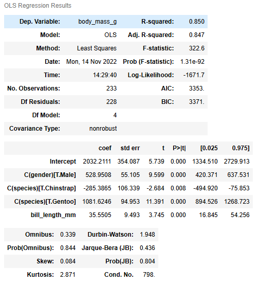
Warnings:
[1] Standard Errors assume that the covariance matrix of the errors is correctly specified.
We can now interpret each of the beta coefficients for each X variable.
C(gender) – Male
Given the name of the variable, we know that the variable was encoded as Male = 1, Female = 0. This means that female penguins are the reference point. If all other variables are constant, then we would expect a male penguin’s body mass to be about 528.95 grams more than a female penguin’s body mass.
C(species) – Chinstrap and Gentoo
Given the names of these two variables, we know that Adelie penguins are the reference point. So, if we compare an Adelie penguin and a Chinstrap penguin, who have the same characteristics except their species, we would expect the Chinstrap penguin to have a body mass of about 285.39 grams less than the Adelie penguin.
If we compare an Adelie penguin and a Gentoo penguin, who have the same characteristics except their species, we would expect the Gentoo penguin to have a body mass of about 1,081.62 grams more than the Adelie penguin.
Bill length (mm)
Lastly, bill length (mm) is a continuous variable, so if we compare two penguins who have the same characteristics, except one penguin’s bill is 1 millimeter longer, we would expect the penguin with the longer bill to have 35.55 grams more body mass than the penguin with the shorter bill.
Disclaimer: Like most of my posts, this content is intended solely for educational purposes and was created primarily for my personal reference. At times, I may rephrase original texts, and in some cases, I include materials such as graphs, equations, and datasets directly from their original sources.
I typically reference a variety of sources and update my posts whenever new or related information becomes available. For this particular post, the primary source was Google Advanced Data Analytics Professional Certificate.