# Standard operational package imports
import numpy as np
import pandas as pd

#  Imports for modeling and evaluation
from sklearn.cluster import KMeans
from sklearn.metrics import silhouette_score
from sklearn.preprocessing import StandardScaler

# (To create synthetic data)
from sklearn.datasets import make_blobs

# Visualization package import
import seaborn as sns
Create the data
In practice, we’d have a dataset of real data, but for simplicity and to help us focus on the modeling itself, we’re going to use synthetic data for this demonstration. We’ll start by creating a random number generator. This is to help with the process of creating reproducible synthetic data. We’ll use it to create clustered data without us knowing how many clusters there are.
# Create random number generator
rng = np.random.default_rng(seed=44)
By calling the random number generator and assigning the result to a variable, we can avoid seeing the true number of clusters our data has. This keeps the “answer” a secret, and will let us use inertia and silhouette coefficients to determine it.
# Create synthetic data w/ unknown number of clusters
centers = rng.integers(low=3, high=7)
X, y = make_blobs(n_samples=1000, n_features=6, centers=centers, random_state=42)
The above steps that generated our synthetic data return two things: X and y. X is an array of the values for the synthetic data itself and y is an array that contains the cluster assignment for each sample in X (represented as an integer).
Right now we’re concerned with X, because it is our mystery data. It’s currently an array, but it’s usually helpful to view your data as a pandas dataframe. This is often how our data will be organized when modeling real-world data, so we’ll convert our data to a pandas df.
# Create Pandas dataframe from the data
X = pd.DataFrame(X)
X.head()| 0 | 1 | 2 | 3 | 4 | 5 | |
|---|---|---|---|---|---|---|
| 0 | -1.534288 | 5.467808 | -6.945988 | 1.403934 | 1.553836 | -7.618236 |
| 1 | -6.681020 | 6.717808 | 2.764396 | 4.460744 | -8.286569 | 10.959708 |
| 2 | -8.678310 | 7.825306 | 3.139699 | 5.609951 | -9.948079 | 8.072149 |
| 3 | -6.667385 | 7.147637 | 2.145505 | 4.712937 | -9.544708 | 11.093248 |
| 4 | -2.753835 | -4.209968 | 0.620345 | -7.439505 | -4.405723 | -2.046149 |
We see that the data has 6 features (columns). This is too many for us to visualize in 2-D or 3-D space. We can’t see how many clusters there are, so we’ll need to use our detective skills to determine this.
Scale the data
Since K-means uses distance between observations and centroids as its measure of similarity, it’s important to scale our data before modeling, if it’s not already scaled. It’s important to scale because K-means doesn’t know what our unit label is for each variable.
Suppose we had data for penguins, and height were measured in meters and weight were measured in grams. Without scaling, significant differences in height would be represented as small numbers, while minor differences in weight would be represented as much larger numbers.
To perform scaling, we’ll use scikit-learn’s StandardScaler. StandardScaler scales each point xᵢ by subtracting the mean value for that feature and dividing by the standard deviation:
x-scaled = (xᵢ – mean(x)) / σ
This ensures that, after scaling, each feature variable has a mean of 0 and variance/standard deviation of 1. There are a number of scaling techniques available, including StandardScaler, MinMaxScaler, Normalizer, and others, each scaling the data in a particular way. There’s no hard rule for determining which method will work best, but with K-means models, using any scaler will almost always result in better results than not scaling at all.
Tip: If our computing environment has sufficient resources, it’s helpful to keep an unscaled copy of our data to use later.
# Scale the data
X_scaled = StandardScaler().fit_transform(X)
X_scaled[:2,:]
array([[-0.03173691, 0.4864719 , -1.32178135, 0.59808997, 1.5703227 ,
-0.88951855],
[-1.05006137, 0.68381835, 0.74465777, 1.2564266 , -0.97057774,
1.92995522]])
Instantiate the model
Now that the data is scaled, we can start modeling. Since we don’t know how many clusters exist in the data, we’ll begin by examining the inertia values for different values of k.
One thing to note is that, by default, scikit-learn implements an optimized version of the K-means algorithm, called K-means++. This helps to ensure optimal model convergence by initializing centroids far away from each other. Because we’re using K-means++, we will not rerun the model multiple times.
We’ll begin by instantiating the model. If we want to build a model that clusters the data into three clusters, we’d set the n_clusters parameter to 3. We’ll also set the random_state to an arbitrary number. This is only so others can reproduce our results.
# Instantiate model
kmeans3 = KMeans(n_clusters=3, random_state=42)
Fit the data
Now that we’ve instantiated the model, the next step is to fit it to the data. We do this by using the .fit() method and passing to it our scaled data.
# Fit model to data
kmeans3.fit(X_scaled)
KMeans(algorithm='auto', copy_x=True, init='k-means++', max_iter=300,
n_clusters=3, n_init=10, n_jobs=None, precompute_distances='auto',
random_state=42, tol=0.0001, verbose=0)
This returns a model object that has “learned” our data. We can now call its different attributes to see inertia, location of centroids, and class labels, among others. We can get the cluster assignments by using the .labels_ attribute. Similarly, we can get the inertia by using the .inertia_ attribute.
print('Clusters: ', kmeans3.labels_)
print('Inertia: ', kmeans3.inertia_)
Clusters: [2 1 1 1 0 0 0 1 1 2 0 1 1 2 1 1 1 1 0 0 0 1 1 1 2 2 0 1 1 0 0 1 0 0 2 2 0
1 1 1 0 1 0 1 1 0 0 2 1 2 0 0 0 2 2 2 0 1 0 2 0 0 0 0 0 0 0 2 0 0 1 0 0 0
1 0 1 2 2 1 2 1 0 2 0 1 2 2 1 2 1 0 2 1 0 2 0 1 1 0 0 1 1 1 1 1 1 0 0 1 2
0 1 0 1 1 0 0 2 0 0 0 1 0 0 1 1 0 2 1 2 2 2 0 1 2 2 0 1 0 0 0 1 2 2 2 0 0
1 0 0 1 0 0 1 1 2 1 2 1 1 0 1 1 1 1 0 0 1 0 1 1 0 1 1 2 1 1 2 2 0 1 0 1 0
1 2 1 2 1 0 0 0 1 1 1 2 2 1 0 1 1 0 1 0 0 0 0 0 2 0 2 1 1 0 2 2 1 0 0 2 0
1 1 1 1 0 0 0 1 2 0 2 1 2 1 2 0 0 1 1 1 2 2 0 0 2 2 2 1 1 1 0 0 0 1 1 1 0
1 0 2 0 1 1 2 2 0 0 1 0 2 1 0 1 1 1 1 0 1 1 0 1 1 0 0 0 0 0 1 2 0 1 0 2 2
0 1 1 0 1 1 1 1 1 1 2 1 2 0 1 1 2 0 0 1 0 1 1 2 1 0 1 1 1 0 0 0 2 2 2 0 2
2 2 1 1 2 1 2 0 1 0 2 1 2 0 1 0 1 1 1 1 0 0 1 0 1 0 0 0 2 1 1 1 1 1 0 0 2
0 1 1 0 1 0 0 1 0 1 2 1 1 0 1 0 0 2 1 0 0 0 2 0 0 1 0 1 0 1 2 1 0 1 1 0 0
2 1 0 0 2 0 0 1 1 1 1 0 1 0 1 1 2 2 0 2 0 0 0 1 1 2 0 1 1 1 0 1 0 1 2 1 0
2 0 0 0 1 0 2 1 0 2 1 1 0 0 0 0 0 1 1 0 1 1 0 1 1 0 0 2 0 2 1 0 0 0 0 2 1
1 0 1 1 2 2 1 0 1 2 2 1 0 1 1 0 0 0 2 1 0 0 1 2 2 0 2 1 0 0 1 1 0 1 0 1 0
0 0 1 1 0 0 1 1 2 1 2 0 0 0 2 1 0 0 0 1 2 2 2 2 2 1 0 2 1 0 1 1 0 2 0 1 2
1 1 1 0 0 1 0 0 0 2 2 1 1 0 0 1 1 2 1 0 1 1 2 1 0 0 0 2 1 2 0 0 2 1 1 0 0
0 0 0 1 1 2 1 2 0 2 0 2 2 1 0 0 1 2 1 2 0 2 1 0 1 0 0 1 1 0 1 1 0 1 1 0 0
1 1 1 1 0 2 0 1 1 0 1 0 0 1 1 0 0 0 2 2 2 0 0 2 1 2 2 0 2 1 1 1 1 1 1 0 2
1 1 0 0 0 1 1 0 1 0 1 0 0 1 0 1 0 1 0 1 0 1 1 0 1 0 1 1 2 0 0 0 1 2 1 0 2
2 1 0 1 1 0 1 1 1 2 1 0 1 1 0 2 1 2 1 0 0 0 1 0 1 2 1 0 1 0 1 1 2 1 1 0 0
0 1 0 0 1 1 0 2 2 1 0 0 0 1 0 0 2 0 2 0 2 0 0 1 1 0 0 0 2 2 0 0 0 2 0 1 2
0 0 0 0 1 2 1 0 1 0 1 2 1 0 0 1 0 2 0 0 1 2 0 1 0 0 2 0 0 1 0 2 1 2 2 1 2
1 0 0 0 0 0 2 2 1 1 0 1 0 1 1 0 1 2 0 2 1 0 0 0 1 1 1 1 1 1 0 2 1 1 1 1 1
0 2 2 2 1 0 0 2 1 1 1 0 0 0 2 0 1 0 0 1 0 0 0 0 0 0 0 2 1 0 1 0 1 1 0 0 1
2 1 1 1 2 0 1 0 0 2 0 2 0 2 1 2 1 2 2 1 1 1 1 0 0 0 1 0 0 2 1 1 1 0 0 1 0
2 1 0 1 0 1 1 1 1 1 1 2 1 2 1 1 2 1 1 0 0 1 1 0 0 0 0 1 1 2 1 1 1 1 1 0 0
0 1 0 2 1 1 1 0 1 2 0 1 2 1 0 0 2 0 0 0 0 1 1 0 0 0 0 0 2 0 1 0 2 2 2 1 0
0]
Inertia: 1748.1488703079513
The .labels_ attribute returns a list of values that is the same length as the training data. Each value corresponds to the number of the cluster to which that point is assigned. Since our K-means model clustered the data into three clusters, the value assigned to each observation will be 0, 1, or 2. Note that the cluster number itself is arbitrary, and serves only as a label.
The .inertia_ attribute returns the sum of the squared distances of samples from their closest cluster center.
Evaluate inertia
This inertia value isn’t helpful by itself. We need to compare the inertias of multiple k values. To do this, we’ll create a function that fits a K-means model for multiple values of k, calculates the inertia for each k value, and appends it to a list.
# Create a list from 2-10.
num_clusters = [i for i in range(2, 11)]

def kmeans_inertia(num_clusters, x_vals):
    '''
    Fits a KMeans model for different values of k.
    Calculates an inertia score for each k value.
    Args:
        num_clusters: (list of ints)  - The different k values to try
        x_vals:       (array)         - The training data
    Returns:
        inertia:      (list)          - A list of inertia scores, one for each \
                                      value of k
    '''
    inertia = []
    for num in num_clusters:
        kms = KMeans(n_clusters=num, random_state=42)
        kms.fit(x_vals)
        inertia.append(kms.inertia_)

    return inertia
# Calculate inertia for k=2-10
inertia = kmeans_inertia(num_clusters, X_scaled)
inertia[3090.3260348468534, 1748.1488703079513, 863.1663243212965, 239.65434758718428, 230.04809652569242, 221.84910615776585, 214.924430018772, 206.49351159542385, 201.31356585907992]
Elbow plot
Now we can plot these values in a simple line graph, with the k values along the x-axis and inertia on the y-axis. This type of plot is called an elbow plot. The “elbow” is usually the part of the curve with the sharpest angle, where the reduction in inertia that occurs when a new cluster is added begins to level off.
# Create an elbow plot
plot = sns.lineplot(x=num_clusters, y=inertia)
plot.set_xlabel("Number of clusters")
plot.set_ylabel("Inertia")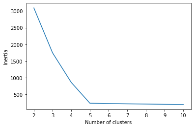
This plot contains an unambiguous elbow at five clusters. Models with more than five clusters don’t seem to reduce inertia much at all. Right now, it seems like a 5-cluster model might be optimal.
Let’s now check silhouette scores. Hopefully the results will corroborate our findings from the assessment of inertia.
Evaluate silhouette score
Unlike inertia, silhouette score doesn’t have its own attribute that can be called on the model object. To get a silhouette score, we have to use the silhouette_score() function that we imported from sklearn.metrics. We must pass to it two required parameters: our training data and their assigned cluster labels. Let’s see what this looks like for the kmeans3 model we created earlier.
# Get silhouette score for kmeans3 model
kmeans3_sil_score = silhouette_score(X_scaled, kmeans3.labels_)
kmeans3_sil_score
0.5815196371994135
This value isn’t very useful if we have nothing to compare it to. Just as we did for inertia, we’ll write a function that compares the silhouette score of each value of k, from 2 through 10.
def kmeans_sil(num_clusters, x_vals):
    '''
    Fits a KMeans model for different values of k.
    Calculates a silhouette score for each k value
    Args:
        num_clusters: (list of ints)  - The different k values to try
        x_vals:       (array)         - The training data
    Returns:
        sil_score:    (list)          - A list of silhouette scores, one for each \
                                      value of k
    '''
    sil_score = []
    for num in num_clusters:
        kms = KMeans(n_clusters=num, random_state=42)
        kms.fit(x_vals)
        sil_score.append(silhouette_score(x_vals, kms.labels_))

    return sil_score
# Calculate silhouette scores for k=2-10
sil_score = kmeans_sil(num_clusters, X_scaled)
sil_score[0.4792051309087744, 0.5815196371994135, 0.6754359269330666, 0.7670656870960783, 0.653416866862045, 0.5281737567081295, 0.3985795104853446, 0.2712146613692562, 0.2759058087446766]
We can plot the silhouette score for each value of k, just as we did for inertia. However, remember that for silhouette score, greater numbers (closest to 1) are better, so we hope to see at least one clear “peak” that is close to 1.
# Create a line plot of silhouette scores
plot = sns.lineplot(x=num_clusters, y=sil_score)
plot.set_xlabel("# of clusters")
plot.set_ylabel("Silhouette Score")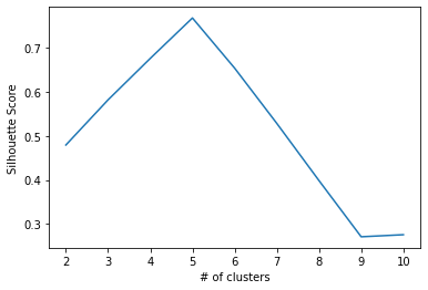
This plot indicates that the silhouette score is closest to 1 when our data is partitioned into five clusters. It confirms what we saw in the inertia analysis, where we noticed an elbow where k=5.
Conclusion
At this point, between our inertia and silhouette score analyses, we can say with a reasonable degree of confidence that it makes the most sense to group our data into five clusters.
Since we used synthetic data for this activity, we can cheat and check to see how many clusters actually existed in our data. We can do this by calling the centers variable, which we created with the random number generator at the beginning of this notebook.
# Verify our findings (only possible when "correct" number of clusters exists)
centers
5
We were right! Just as we predicted, there are indeed five distinct clusters in our data. We were able to deduce this by using inertia and silhouette score.
Further analysis
Although we know that five clusters is the best grouping for the data, the work is far from done. At this point, we’ll instantiate a new K-means model with n_clusters=5 and fit it to our data.
Note that if we had saved all the models that we fit above for different values of k, we wouldn’t need to refit a model now, we could just call that model from earlier. But since it wasn’t saved, we must fit another model.
# Fit a 5-cluster model to the data
kmeans5 = KMeans(n_clusters=5, random_state=42)
kmeans5.fit(X_scaled)
KMeans(algorithm='auto', copy_x=True, init='k-means++', max_iter=300,
n_clusters=5, n_init=10, n_jobs=None, precompute_distances='auto',
random_state=42, tol=0.0001, verbose=0)
print(kmeans5.labels_[:5])
print('Unique labels:', np.unique(kmeans5.labels_))
[2 3 3 3 4]
Unique labels: [0 1 2 3 4]
Now that we have our labels, it’s important to understand what they mean and decide whether this clustering makes sense for our use case. Here’s where it helps to keep our unscaled data from the beginning. We can assign a new column to the original unscaled dataframe with the cluster assignment from the final K-means model.
# Create new column that indicates cluster assignment in original dataframe
X['cluster'] = kmeans5.labels_
X.head()| 0 | 1 | 2 | 3 | 4 | 5 | cluster | |
|---|---|---|---|---|---|---|---|
| 0 | -1.534288 | 5.467808 | -6.945988 | 1.403934 | 1.553836 | -7.618236 | 2 |
| 1 | -6.681020 | 6.717808 | 2.764396 | 4.460744 | -8.286569 | 10.959708 | 3 |
| 2 | -8.678310 | 7.825306 | 3.139699 | 5.609951 | -9.948079 | 8.072149 | 3 |
| 3 | -6.667385 | 7.147637 | 2.145505 | 4.712937 | -9.544708 | 11.093248 | 3 |
| 4 | -2.753835 | -4.209968 | 0.620345 | -7.439505 | -4.405723 | -2.046149 | 4 |
Now, we can perform analyses on the different clusters to see what makes them different from one another. The reason we’d look at cluster assignments with the unscaled data is because it’s easier to relate to the unit measures. This is often a useful technique for analyzing our data, but it may also make sense to look at our cluster assignments on the scaled data, depending on our use case.
Note that in many cases, it’s not always clear what differentiates one cluster from another, and it takes a lot of work to determine whether or not it makes sense to cluster our data a given way. This is where expertise and domain knowledge are very valuable.
Predicting on new data
This is not applicable to all clustering tasks, but it’s now possible to take in new data and predict a cluster assignment using our final model.
To demonstrate this, we’ll need a new observation, one that was not contained in our original data. We can create this with the random number generator that we used at the beginning of the notebook.
# Create a new observation (for demonstration)
new_observation = rng.uniform(low=-10, high=10, size=6).reshape(1, -1)
new_observation
array([[-4.8377385 , -1.88458544, 9.38367896, -6.7536575 , 7.14587347,
-6.73909458]])
Just as before, we must scale this new data the same way we did earlier. This means that we need to subtract the mean of the training data and divide by the standard deviation of the training data. If we forgot to scale here we’d get invalid results, because our model would be trained on scaled data while the new data going into it would be unscaled.
Here, we must re-instantiate a scaler and fit it to the original data, because we didn’t save the scaler object itself when we performed scaling above. We fit and transformed the data in a single line of code, without saving the fit scaler object.
Above, if instead of:X_scaled = StandardScaler().fit_transform(X)
we had written:scaler = StandardScaler()fit.(X)X_scaled = scaler.transform(X)
then we could have reused scaler in this next step without having to assign it.
# Instantiate the scaler and fit it to the original X data
scaler = StandardScaler().fit(X.iloc[:,:-1])

# Apply the scaler to the new observation
new_observation_scaled = scaler.transform(new_observation)
new_observation_scaled
array([[-0.68535259, -0.67430308, 2.1532887 , -1.15878741, 3.01424824,
-0.75609599]])
We can use the .predict() method of our kmeans5 model to predict a cluster assignment by passing to it the new observation. In this case, we only have a single observation, but it’s also possible to pass an array of new data as an argument, and it would return an array of cluster predictions.
# Predict cluster assignment of new_observation
new_prediction = kmeans5.predict(new_observation_scaled)
new_prediction
array([4], dtype=int32)
The model has assigned this new observation to cluster 4.
Calculating the distance to each centroid
The KMeans model also lets us access the distances of observations from each centroid. For new data, we can do this using the .transform_ method of the fit model object.
# Calculate distances between new data and each centroid
distances = kmeans5.transform(new_observation_scaled)
distances
array([[5.11675395, 4.55233304, 4.14567617, 5.95732403, 3.46792667]])
Notice that the .transform_ method returns an array. In this case, we gave the model a single new data point, and it returned an array of five numbers (because our model has five clusters). Each value in the array represents the distance between new_observation_scaled and the centroid of the cluster at that index.
So, the distance between new_observation_scaled and the centroids of:
Cluster 0 = 5.12
Cluster 1 = 4.55
Cluster 2 = 4.15
Cluster 3 = 5.96
Cluster 4 = 3.47
The shortest distance is 3.47, between new_observation_scaled and cluster 4’s centroid. This is why the point was assigned to cluster 4 when we used the .predict() method above.
Why is this useful?
One situation for which being able to assign new points to clusters is useful is when we have a deployed model that was trained on huge amounts of data, and it must process new data as it comes in on a case-by-case basis.
For example, suppose we have a marketing program that sends out different promotional emails to different customers, depending on their engagement patterns with our brand. When we get a new customer, we could use a clustering model to assign them to an appropriate marketing campaign, so they see promotions that are most appropriate for them.
Also, both the cluster predictions and the distance measurements to centroids can be used as new features in supervised learning models. We can take the training data of a supervised learning problem and cluster it, then use either the cluster assignments or the distance matrices as engineered predictive features to improve the predictive power of a supervised learning model.
Disclaimer: Like most of my posts, this content is intended solely for educational purposes and was created primarily for my personal reference. At times, I may rephrase original texts, and in some cases, I include materials such as graphs, equations, and datasets directly from their original sources.
I typically reference a variety of sources and update my posts whenever new or related information becomes available. For this particular post, the primary source was Google Advanced Data Analytics Professional Certificate program.