Previously we got our equations for optimal m and b, and now let’s put all of those into practice. So far we get these:
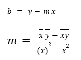
The last one we can see in some books as:
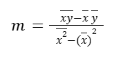
(that’s just multiplying the numerator and denominator by negative one)
Sample 1
Assume we have the following points:
(1, 2)
(2, 1)
(4, 3)
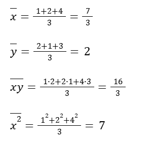
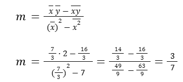
Let’s put all these together and find the slope.
Now, let’s find the y-intercept.
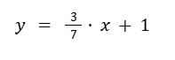
So, we have the equation for our line.
Sample 2
Let’s find the equation for the regression line that fits best to the data points below. And then, let’s calculate how good of a fit it is, using an r-squared.
(-1, -1)
(-2, -3)
(1, 2)
(4, 3)
Let’s remember three equations first:
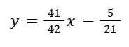
1- The line is going to have the equation y = mx + b.
2- The slope of that line, the one that best minimizes the squared distance to each of those data points, is going to be:
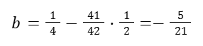
3- The y-intercept (b) is going to be:
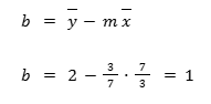
b = ȳ – mx̄
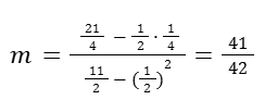
Let’s start with the components to get the m.
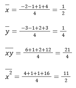
So the slope would be:
And the b, y-intercept, is going to be:
Our regression is going to be:
Calculating R-squared
Now, let’s calculate the r-squared for this line to check how good of a fit it is. How much of the total variation in the y-values can be explained by the variation in the x-values?
We can use a spreadsheet to calculate.
| x | y | y-predicted | squared error with line | squared error from mean y |
| -2 | -3 | -2.1905 | 0.6553287982 | 10.5625 |
| -1 | -1 | -1.2143 | 0.04591836735 | 1.5625 |
| 1 | 2 | 0.7381 | 1.592403628 | 3.0625 |
| 4 | 3 | 3.6667 | 0.4444444444 | 7.5625 |
| Σ = 2.738095238 | Σ = 22.75 |
We computed:
SELINE = 2.74 and SEȳ = 22.75
First one is essentially the error that the line does not explain, and the second one is the total error, eg. total variation of the numbers.
So if we want to know the percentage of the total variation that is not explained by the line, we divide the first one with the second one.
2.74 / 22.75 = 0.12 is the percentage of total variation NOT explained by variation in x.
Our r-squared, which is the percent of the total variation that is explained by x, is going to be
1 – 0.12 = 0.88.
A way to interpret this, is that 88% of the total variation of those y values is explained by the variation in x.
Disclaimer: Like most of my posts, this content is intended solely for educational purposes and was created primarily for my personal reference. At times, I may rephrase original texts, and in some cases, I include materials such as graphs, equations, and datasets directly from their original sources.
I typically reference a variety of sources and update my posts whenever new or related information becomes available. For this particular post, the primary source was Khan Academy’s Statistics and Probability series.