Logistic regression is a technique that models a categorical dependent variable (Y) based on one or more independent variables (X). We’ll focus here mostly on binomial logistic regression.
Binomial logistic regression is a technique that models the probability of an observation falling into one of two categories based on one or more independent variables.
Find the best logistic regression model for our data
Just like any other statistical method, we have to make assumptions about the data to have confidence in the results. Assumptions of binomial logistic regression are:
1. Linearity
There should be a linear relationship between each X variable and the logit of the probability that Y equals 1.
The linearity assumption is the key assumption that explains how we can estimate a logistic regression model that fits the data best. To understand logit, we must first define the odds. The odds of a given probability p is:
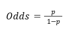
We can think of the equation as the probability of P occurring divided by the probability of P not occurring.
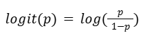
The logit (log-odds) function is the logarithm of the odds of a given probability. So the logit of probability P is:
Logit is the most common link function used to linearly relate the X variables to the probability of Y.
By assuming that there is a linear relationship between the X variables and the logit of the probability that Y=1 (our outcome of interest), we can then find some beta coefficient that explains the data we’ve observed.
We can write the logit of P in terms of the X variables:
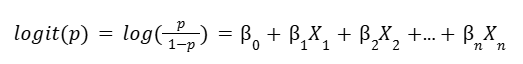
Where n is the number of independent variables we are considering in our model.
Like linear regression, we don’t want just any set of beta coefficients. We want the best set of beta coefficients to make sure our model fits the data. In linear regression, we minimize the sum of squared residuals (which is a measure of error), to figure out the best model. In logistic regression, we’ll often use maximum likelihood estimation to find the best logistic regression model.
Maximum likelihood estimation (MLE) is a technique for estimating the beta parameters that maximize the likelihood of the model producing the observed data.
We can think of likelihood as the probability of observing the actual data, given some set of beta parameters.
2. Independent observations
This assumption relates to how the data was collected. Because the observations are assumed to be independent, we can say:
P(A and B) = P(A) * P(B)
Therefore, if we have n basketball players on our team, we can calculate the likelihood of observing the outcome for each player, and then multiply all of the likelihoods together to determine the likelihood of observing all of the sample data.
The best logistic regression model estimates the set of beta coefficients that maximizes the likelihood of observing all of the sample data.
3. No multicollinearity
We assume that there is little to no multicollinearity between the independent variables. If we include multiple X variables, they should not be highly correlated with one another, just like with linear regression.
4. No extreme outlier
Outliers are a complex topic in regression modeling and can be detected after the model is fit. Sometimes it is appropriate to transform or just keep the variables to maintain model validity. Other times it can be appropriate to remove outlier data.
Disclaimer: Like most of my posts, this content is intended solely for educational purposes and was created primarily for my personal reference. At times, I may rephrase original texts, and in some cases, I include materials such as graphs, equations, and datasets directly from their original sources.
I typically reference a variety of sources and update my posts whenever new or related information becomes available. For this particular post, the primary source was Google Advanced Data Analytics Professional Certificate.