Minimizing the squared error of regression line

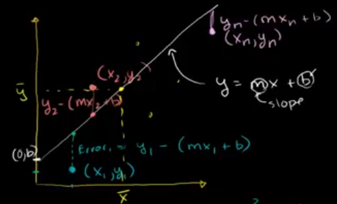
Using the formula y=mx+b, we can write the total squared error of a line as:

SE_line = (y₁-(mx₁+b))² + (y₂-(mx₂+b))² + . . . + (y_n-(mx_n+b))²

We want to find the m and b that minimizes the SE line.

Proof of minimizing the squared error to regression line

SE_line = y₁² – 2y₁(mx₁+b) + (mx₁+b)²
           + y₂² – 2y₂(mx₂+b) + (mx₂+b)²
. . . 
          + y_n² – 2y_n(mx_n+b) + (mx_n+b)²

SE_line = y₁² – 2y₁mx₁ – 2y₁b + m²x₁² + 2mx₁b + b²
           + y₂² – 2y₂mx₂ – 2y₂b + m²x₂² + 2mx₂b + b²
. . . 
           + y_n² – 2y_nmx_n – 2y_nb + m²x_n² + 2mx_nb + b²

We can write all the above (by factoring out some of the parts) as:

= (y₁² + y₂² + … + y_n²) – 2m(x₁y₁ + x₂y₂ + … + x_ny_n) – 2b(y₁ + y₂ + … + y_n)
+ m²(x₁² + x₂² + … + x_n²) + 2mb(x₁ + x₂ + … + x_n) + nb²

The mean of the y-squared is:

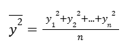
That we can write as:

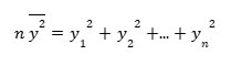
Similarly we can do:

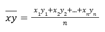
Which can be written as:

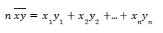
Now, our main equation can be written as:

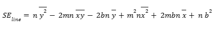
Optimizing the expression

Until now it was a hard core algebra stage, now we actually want to optimize this. Hence, we want to find the m and the b values that minimize the above expression.

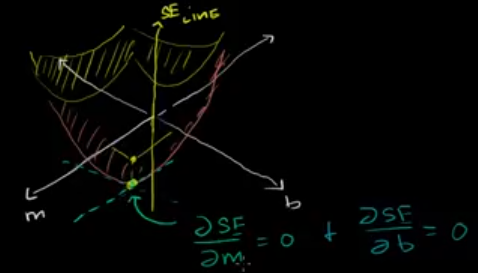
To help visualize it, we’re going to start breaking into a little bit of 3-d calculus (It won’t be difficult if you’ve done any partial derivatives). This (above) is a surface in 3-d.

If we say that we have the x and y data points (we assume that we have them and those are actual numbers), everything here is a constant except for the m’s and the b’s.

Imagine, we have m-axis and b-axis (like the x-y axes) and the vertical axis (like z-axis), to be the squared-error (of the line).

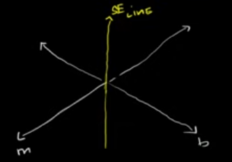
Any combination of m and b’s will give us a point. If we do that for all of the combinations of m’s and b’s, we’re going to get a surface. That’s going to look like a kind of a bowl, or a 3d parabola.

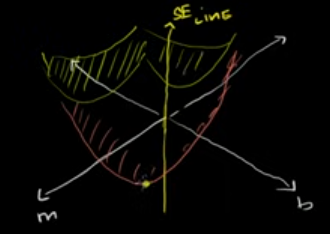
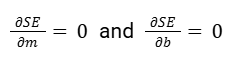
We’re trying to find the m and b values that minimize the value on the surface. To do that, we need to find the partial derivative of SE-line with respect to m and with respect to b and set both of them equal to zero. 

Because the minimum point on the surface is going to occur when the slope with respect to m and the slope with respect to b is zero.

So at that point, the partial derivative of our squared error with respect to m is going to be equal to 0. And the partial derivative of our squared error with respect to b is going to be equal to 0.

Partial derivative 

Meaning, the slope in the direction of m (that’s the partial derivative with respect to m) is going to be flat. And, the slope in the direction of b (that’s the partial derivative with respect to b) is also going to be flat. That is our minimum point.

Now, let’s remember our equation.

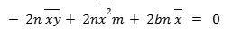
When we take the partial derivative with respect to m, the only variable that matters is the m.

n y² part is constant (with respect to m), since there is no m there. So its partial derivative with respect to m is 0.

Derivative of 2mn xy with respect to m, is like the coefficients on the m. So it is -2n xy.

So we get:

Now when do the same thing with respect to b, we get:

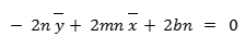
Since 0 is divisible by anything, we can divide the top equation by 2n and we’ll be left with:

So if we find the m and the b values that satisfy the system of equations (above), we have minimized the squared error.

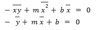
We can rewrite them as:

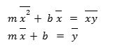
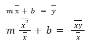
We can actually get both of these into mx + b form.

From the second equation we can tell that the mean of x and the mean of y, (x̄, ȳ) lies on the line. Since the equation of the line is y = mx + b.

Now we can ask ourselves: What’s another point on the line?
Because if we know two points on the line, we know what the equation of the line is going to be.

Let’s try to get the first one also in mx + b form, by dividing them by the mean of the x.

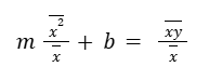
So, another point on the (optimal) line is going to be the point:

Two points (x̄, ȳ) and  both lie on the best fitting line, based on how we’re measuring a good fit, which is the squared distance. These are on the line that minimize that squared distance.

The optimal m and b

Let’s solve for m first. This means that we want to cancel out the b’s. We can do that by subtracting the bottom equation from the top equation.

So we get:

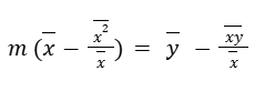
Or another way to put that out:

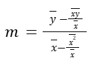
It’s the same thing if we found the slope between those two points(x̄, ȳ) and . Or we can say: Change in y, over the change in x’s.

If we like to simplify above (by multiplying the numerator by the mean of the x’s), we get:

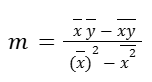
Now, we can solve for b, by substituting (this m above) back into the equation.

b = ȳ – mx̄

So, we take our data points, find the mean of the x’s, the mean of the y’s, the mean of the xy’s and the mean of the x’s-squared. Then we find our m. And, we can substitute back in the above equation and find our b. Then we have our actual optimal line.

---

Disclaimer: Like most of my posts, this content is intended solely for educational purposes and was created primarily for my personal reference. At times, I may rephrase original texts, and in some cases, I include materials such as graphs, equations, and datasets directly from their original sources.

I typically reference a variety of sources and update my posts whenever new or related information becomes available. For this particular post, the primary source was Khan Academy’s Statistics and Probability series.