Multivariate Analysis of Corolla Dataset

---

OVERVIEW

---

1 Introduction

Toyota Corolla dataset was given us as a practice set during the openHPI‘s Data Science Bootcamp 2023. It was introduced under the ‘EDA and Statistical Analysis’ section to demonstrate MVA studies. It was not an assignment but part of the lecture. Yet I wanted to play around and use the dataset to answer some other questions and then shared my analysis in the forum with the title ‘Getting charmingly lost in the Corolla dataset‘.

The instructors provided me useful feedback but some questions were still not answered (you’ll find them below). So I decided to dive deeper to hopefully find some explanations and (even if not) to gain further knowledge and skills on data analysis processes.

It’s better to underline that I am at the entry level in data science and I am aware of other methods and models that may fit better here. But I limited myself within MVA and Linear Regression.

I hope this work of mine will demonstrate how I approach to a dataset that has a wide-range of variables and what kind of reasonings I developed to some certain data analysis issues.

1.1 The Origin of the Dataset

Although there are a bunch of studies regarding this exact Corolla dataset on the web, it is not possible to find the initial source of it, at least publicly. I spent hours trying to find out where this dataset comes from, by whom it was collected and where it was shared. I did so, because I believe every data-related research should start with questioning the data itself. Besides, the unanswered questions in my initial analysis that I mentioned above might be a result of a dummy set, as the instructors were not able to clarify the source of it.

Unfortunately I did not find the main source but I guess I found where this set first appeared. If you want to read more about this research of mine, you can visit my post here.

1.2 What is this Dataset about?

I’ll stick with the only description that is available online:

“The file ToyotaCorolla.xls contains data on used cars (Toyota Corolla) on sale during late summer of 2004 in The Netherlands. It has 1436 records containing details on 38 attributes, including Price, Age, Kilometers, HP, and other specifications. The goal is to predict the price of a used Toyota Corolla based on its specifications.“

In the DS Bootcamp we were using this dataset for the same purpose. We were giving a set of values and were trying to predict the price. As I mentioned above, afterwards I came up with different questions just to practice the methods that were shown to us.

Let’s have a quick look at those attributes:

import numpy as np 
import pandas as pd 
import seaborn as sns 
import matplotlib.pyplot as plt

df = pd.read_csv('/kaggle/input/toyotacorolladataset/ToyotaCorolla.csv')

df.info()

<class 'pandas.core.frame.DataFrame'>
RangeIndex: 1436 entries, 0 to 1435
Data columns (total 39 columns):
 #   Column             Non-Null Count  Dtype 
---  ------             --------------  ----- 
 0   Id                 1436 non-null   int64 
 1   Model              1436 non-null   object
 2   Price              1436 non-null   int64 
 3   Age_08_04          1436 non-null   int64 
 4   Mfg_Month          1436 non-null   int64 
 5   Mfg_Year           1436 non-null   int64 
 6   KM                 1436 non-null   int64 
 7   Fuel_Type          1436 non-null   object
 8   HP                 1436 non-null   int64 
 9   Met_Color          1436 non-null   int64 
 10  Color              1436 non-null   object
 11  Automatic          1436 non-null   int64 
 12  CC                 1436 non-null   int64 
 13  Doors              1436 non-null   int64 
 14  Cylinders          1436 non-null   int64 
 15  Gears              1436 non-null   int64 
 16  Quarterly_Tax      1436 non-null   int64 
 17  Weight             1436 non-null   int64 
 18  Mfr_Guarantee      1436 non-null   int64 
 19  BOVAG_Guarantee    1436 non-null   int64 
 20  Guarantee_Period   1436 non-null   int64 
 21  ABS                1436 non-null   int64 
 22  Airbag_1           1436 non-null   int64 
 23  Airbag_2           1436 non-null   int64 
 24  Airco              1436 non-null   int64 
 25  Automatic_airco    1436 non-null   int64 
 26  Boardcomputer      1436 non-null   int64 
 27  CD_Player          1436 non-null   int64 
 28  Central_Lock       1436 non-null   int64 
 29  Powered_Windows    1436 non-null   int64 
 30  Power_Steering     1436 non-null   int64 
 31  Radio              1436 non-null   int64 
 32  Mistlamps          1436 non-null   int64 
 33  Sport_Model        1436 non-null   int64 
 34  Backseat_Divider   1436 non-null   int64 
 35  Metallic_Rim       1436 non-null   int64 
 36  Radio_cassette     1436 non-null   int64 
 37  Parking_Assistant  1436 non-null   int64 
 38  Tow_Bar            1436 non-null   int64 
dtypes: int64(36), object(3)
memory usage: 437.7+ KB

Below I’ll go through every single column one by one. Therefore I won’t repeat the description of them here, but I’ll provide them on each section.

2 Problem Statement

After some good amount of UX practices I learned my lesson that every research should start with a problem statement. So I had some hypothesis that some features of a car such as air conditioning or powered windows should get more important when the car gets older. Following this I came up with the question below:

“What (feature) becomes more important
(~valuable, pricey) when a car is aging?”

2.1 Setting the boundaries: What is old?

But first, I needed to be sure that this dataset contains information related to that statement. If this would be a real-life study, then that statement should’ve come with more clear direction, like ‘what gets important after 10 (or whatever the business goal is) years?’. Here I had to draw my limits within the dataset itself, because if this particular dataset had only 10% of cars that are older than -say- 3 years old, then it wouldn’t make much sense to study this statement with this set. So I tried different years:

(The column ‘Age_08_04’ represents age in months as in August 2004)

three_years = df[(df.Age_08_04 >= 36)]
four_years = df[(df.Age_08_04 >= 48)]
five_years = df[(df.Age_08_04 >= 60)]
six_years = df[(df.Age_08_04 >= 72)]

three_years_old = len(three_years)
four_years_old = len(four_years)
five_years_old = len(five_years)
six_years_old = len(six_years)

total_cars = len(df)

print(f"Number of cars older than 3 years: {three_years_old}, and they are {three_years_old/total_cars:.2f}%")
print(f"Number of cars older than 4 years: {four_years_old}, and they are {four_years_old/total_cars:.2f}%")
print(f"Number of cars older than 5 years: {five_years_old}, and they are {five_years_old/total_cars:.2f}%")
print(f"Number of cars older than 6 years: {six_years_old}, and they are {six_years_old/total_cars:.2f}%")

Number of cars older than 3 years: 1215, and they are 0.85%
Number of cars older than 4 years: 1034, and they are 0.72%
Number of cars older than 5 years: 754, and they are 0.53%
Number of cars older than 6 years: 319, and they are 0.22%

Targetting the 5 years and older cars sounds good, since they cover almost the half of the whole dataset.

2.2 Summary of my Initial Analysis

To be able to explain why I was in need of a new and deeper analysis, I better provide a short summary of the results from that first analysis.

I’ve chosen 7 variables, which estimated below coefficients in the table.*
(*They were slightly different, because the dataset they provided had 1427 rows in total, unlike the original set with 1436 rows.)

|-------------|-----------|
| hp          |     51.65 | 
| automatic   |    727.40 | 
| doors       |    473.05 | 
| airco       |   2045.85 | 
| pwr windows |     954.6 | 
| radio       |    -39.73 | 
| tow bar     |   -1548.8 |

(a sample reading of this table would be: 
every bit of hp would bring 51.65 euros to the price of a car, 
while having a radio would minus the price by 39.73 euros)

These results were for the whole set. After that, I got the results for the older cars to compare them and at the end I’ve had such questions and notes:

1- I’ve chosen variables that seemed to me to have a potential for a noteworthy-effect on the price, especially for the older cars, but I was not sure how to choose variables accurately.

• Shortly speaking, it’s mostly about the domain-knowledge. One needs a good understanding of the domain and the problem statement as well.
• This time, on this analysis I’ll go through every single column to come up with a better set of variables. I’ll chose them based on the data they carry, rather than relying on my guts.

2- After the comparison, some results made sense but some not. Why having an additional feature like a radio or a tow bar would effect the price negatively?

• For the radio, I’ve had a thesis that it might be caused by people’s expectations for a better feature, like a media screen or a CD player. When I’ve checked them through I’ve understood that I might be right on this. This claim will remain at the end of this analysis as well.
• However for the tow bar, I could not understand the reasons behind. Nor the instructors could. They’ve suggested that this set might be a dummy one. At the end of this analysis I’ll have an explanation how a tow bar can effect the price negatively (and this set indeed could be a real one).

3- Back then I did not realize but changing the variables in the regression model dramatically effects the results. I understood that the digits in the table above are extreme and they get ‘milder’ when other variables are introduced into the equation. I have reached to a sense that some variables are being ‘forced’ to carry the negative effect stronger, if there is no other variables that has also negative effect on the overall price.

• Close to the end of this analysis I’ll demonstrate this as well.

3 EDA & Data Cleaning

Alright, let me roll up my sleeves. The EDA phase will be in three steps:

• First, I’ll check every single column and try to understand the dataset better. Meanwhile I’ll do some necessary cleaning & tidying up. I’ll eliminate some columns that I think won’t serve the problem statement.
• Then, I’ll go deeper and investigate the ones that I could not classify at the first round. I’ll double check the other ones as well.
• Lastly, there will be additional eliminations that will be based on tons of iterations. (This is highly related to the issue that I mentioned above in the 3rd note)

3.1 Basic EDA

This is the first step of the EDA, going through all columns of this dataset.

3.1.1 Id

df.Id.describe()

count    1436.000000
mean      721.555014
std       416.476890
min         1.000000
25%       361.750000
50%       721.500000
75%      1081.250000
max      1442.000000
Name: Id, dtype: float64

The Id column starts from 1 and ends at 1442, but this dataset has 1436 rows in total. None of the dataset I’ve came across in internet during my research had those missing 6 rows. It looks like the author at the very beginning dropped them out. Anyway, this column won’t serve my goal.

3.1.2 Model

This column shows the models of the Corollas. It could be interesting to study models and their performances, but without a proper direction it is very hard to cluster them correctly, since there are 319 unique values in there. Besides, the names of the models hold some information that are already available within this dataset, such as engine size or number of doors. This column also won’t be used in the equation.

df.Model.describe()

count                                                  1436
unique                                                  319
top       TOYOTA Corolla 1.6 16V HATCHB LINEA TERRA 2/3-...
freq                                                    109
Name: Model, dtype: object

3.1.3 Price

(Offer Price in Euros)

This is my dependent variable. Let’s check what’s inside.

df.Price.describe()

count     1436.000000
mean     10730.824513
std       3626.964585
min       4350.000000
25%       8450.000000
50%       9900.000000
75%      11950.000000
max      32500.000000
Name: Price, dtype: float64

sns.histplot(df["Price"])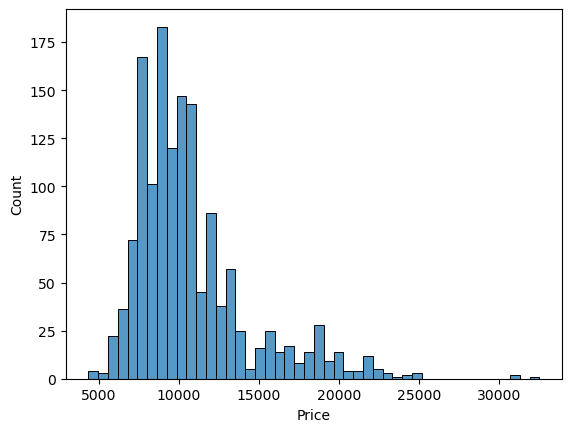

expensive_cars = df[df['Price'] >= 25000]
len(expensive_cars)

3

There is only 3 cars that cost more than 25k each and most of the cars are clustered between around 8k-12k euros.

3.1.4 Age

(Age in months as in August 2004)

The name of the column reflects its description. Let me simplify the name first.

df.rename(columns={'Age_08_04':'Age'}, inplace=True)

df.Age.describe()

count    1436.000000
mean       55.947075
std        18.599988
min         1.000000
25%        44.000000
50%        61.000000
75%        70.000000
max        80.000000
Name: Age, dtype: float64

This dataset has even a one-month-old car, let’s check the distribution. I’ll use years to demonstrate.

x = df["Age"] / 12
plt.xlabel('Years')
sns.histplot(x)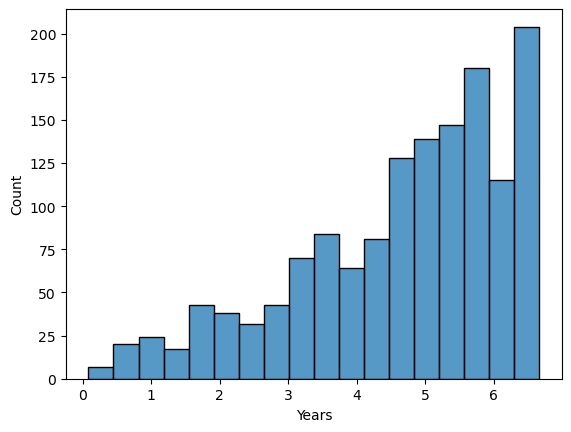

This dataset holds cars that are less than 7 years old and the Age distribution is left skewed.

3.1.5 Mfg_Year & Mfg_Month

(Manufacturing Year & Month)

df.Mfg_Year.describe()

count    1436.000000
mean     1999.625348
std         1.540722
min      1998.000000
25%      1998.000000
50%      1999.000000
75%      2001.000000
max      2004.000000
Name: Mfg_Year, dtype: float64

Manufacturing year and month are just a detailed version of the ‘Age’ column, we can say. I just double checked the digits, which look consistent with the ‘Age’. I can continue with the ‘Age’ only, without these two columns.

3.1.6 KM

(Accumulated Kilometers on odometer)

df.KM.describe()

count      1436.000000
mean      68533.259749
std       37506.448872
min           1.000000
25%       43000.000000
50%       63389.500000
75%       87020.750000
max      243000.000000
Name: KM, dtype: float64

We have a car that was driven only 1 km, and the KM distribution below is right skewed.

sns.histplot(df["KM"])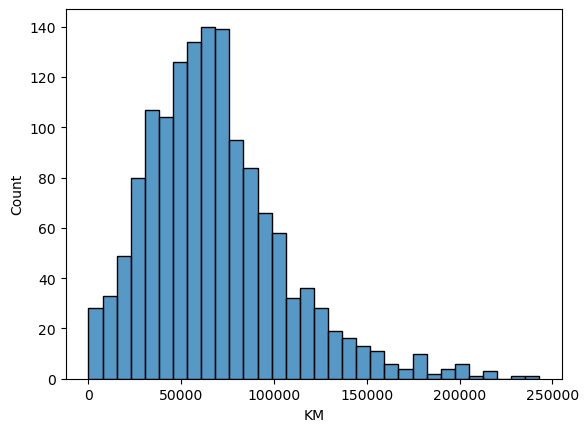

less_used_cars = df[df['KM'] < 10000]
len(less_used_cars)

33

We have 11 cars that are less than 1k-km driven and 33 that are less than 10k-km. For this analysis I won’t do anything about the outliers, unless they are indicators of a poor data entry.

3.1.7 Fuel_Type

sns.histplot(df["Fuel_Type"])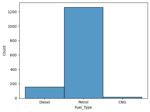

Unfortunately this is the only column about the fuel. It would be nicer to have information about the fuel consumption. Since the petrol type dominates this field, it won’t be helpful to consider this column for older and newer cars seperately, simply bacause the values wouldn’t be fairly distributed.

3.1.8 HP

(Horse Power)

df.HP.describe()

count    1436.000000
mean      101.502089
std        14.981080
min        69.000000
25%        90.000000
50%       110.000000
75%       110.000000
max       192.000000
Name: HP, dtype: float64

sns.histplot(df["HP"])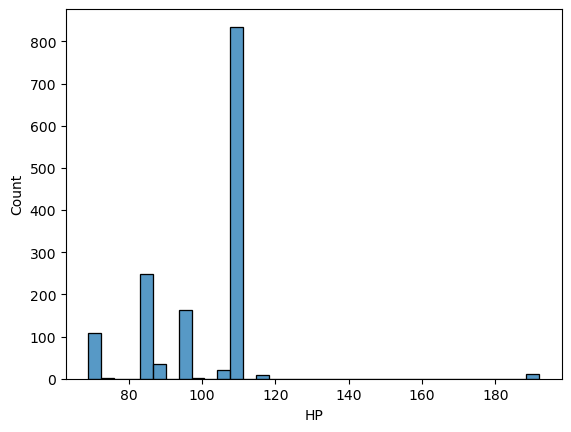

More than half of the cars have 110 hp and mostly they are in less-than-120 range. But there are some very ‘strong’ engines too, let me check them as well, even though I would not touch them.

powered_up = df[df['HP'] > 120]
len(powered_up)

11

df.HP.value_counts()

110    835
86     249
97     164
72      73
90      36
69      34
107     21
192     11
116      9
98       2
71       1
73       1
Name: HP, dtype: int64

3.1.9 Met_Color

Metallic Color (Yes=1, No=0)

Since this is a boolean type, I’ll skip the chart.

df["Met_Color"].value_counts()

1    969
0    467
Name: Met_Color, dtype: int64

Around two-thirds of cars come with a metallic color. For now, I’ll keep them.

3.1.10 Color

Color is a categorical area and I am not sure how I can put it into my numerical MVA. But anyway, it is an interesting topic and color indeed is an important factor for a car, hence its price and probability to be sold fast. I’ll at least check the distribution first.

df["Color"].value_counts()

Grey      301
Blue      283
Red       278
Green     220
Black     191
Silver    122
White      31
Violet      4
Yellow      3
Beige       3
Name: Color, dtype: int64

Said those, I am a bit surprized how there are that few white cars in this set. Where I am from, the white color for a car is the top choice and people almost always refer it as “easy to sell color”. Even though, I wouldn’t add ‘color’ into my equation, I’d like to investigate them further. (You’ll see that I’ll have a guess on white color as well.) (A second note: Where I am from or my experiences are not important, every bit of data should be considered within its original context.)

3.1.11 Automatic

Automatic (Yes=1, No=0)

df["Automatic"].value_counts()

0    1356
1      80
Name: Automatic, dtype: int64

Considering that this data claims to be collected in 2004, it is not surprizing that automatic gear was not that popular yet. If there would be more cars with automatic gear in this dataset, it would worth to examine, but they are so few to be considered.

(After bunch of iterations I’ll put this column back in the equation. I’ll mention about this on further steps.)

3.1.12 CC

(Cylinder Volume in cubic centimeters)

df.CC.describe()

count     1436.00000
mean      1576.85585
std        424.38677
min       1300.00000
25%       1400.00000
50%       1600.00000
75%       1600.00000
max      16000.00000
Name: CC, dtype: float64

That max amount is obviously not a valid input. But let’s check how many we have such high values.

high_cc = df[df['CC'] > 1600]
len(high_cc)

167

That’s a lot. Let’s check what’s within those 167 cars.

df[df['CC'] > 1600].CC.describe()

count      167.000000
mean      2048.892216
std       1087.889163
min       1800.000000
25%       1900.000000
50%       2000.000000
75%       2000.000000
max      16000.000000
Name: CC, dtype: float64

Looks like the highest volume is 2000, without that 16k. Let’s check this one out.

high_cc = df[df['CC'] > 2000]
len(high_cc)

1

Yes it is. It looks like 16k is a typo. Let’s correct it.

df['CC'] = df['CC'].replace(16000, 1600)

df.CC.describe()

count    1436.000000
mean     1566.827994
std       187.182436
min      1300.000000
25%      1400.000000
50%      1600.000000
75%      1600.000000
max      2000.000000
Name: CC, dtype: float64

Looks good, but let me investigate deeper.

df["CC"].value_counts()

1600    846
1300    248
1400    164
2000    119
1900     30
1800     14
1598      4
1587      4
1995      2
1398      2
1332      2
1975      1
Name: CC, dtype: int64

When we talk about the volume of an engine, we don’t need to count every single CC (at least for such analysis). That’s why, those volumes (that are listed above under 1800) can easily be transformed to the nearest 100s.

df["CC"] = df["CC"].round(-2)

df["CC"].value_counts()

1600    854
1300    250
1400    166
2000    122
1900     30
1800     14
Name: CC, dtype: int64

That looks far better, let’s check the graph too.

sns.histplot(df["CC"])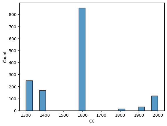

3.1.13 Doors

(Number of doors)

The number of doors, here, I believe can be taken as the indicator for the size of the car. Let’s check how many options we have.

sns.histplot(df["Doors"])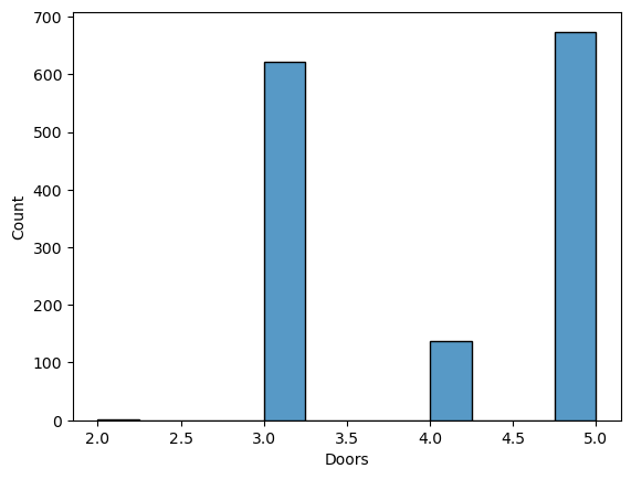

df["Doors"].value_counts()

5    674
3    622
4    138
2      2
Name: Doors, dtype: int64

I don’t know what’s the difference between the 2 and 3 door cars but I won’t try to find this one out, since we have only two of them. I’ll keep this column into my equation for checking the size’s effect on the price.

3.1.14 Cylinders

(Number of cylinders)

df["Cylinders"].value_counts()

4    1436
Name: Cylinders, dtype: int64

All of the cars have 4 cylinders. I don’t need them in my equation.

3.1.15 Gears

(Number of gear positions)

df["Gears"].value_counts()

5    1390
6      43
3       2
4       1
Name: Gears, dtype: int64

Similar to not-having-an-automatic gear, the gears column is also dominated by one value. Almost all cars have 5 gear positions, so it won’t help me much to consider them to compare older and newer cars.

3.1.16 Quarterly_Tax

(Quarterly road tax in Euros)

df.Quarterly_Tax.describe()

count    1436.000000
mean       87.122563
std        41.128611
min        19.000000
25%        69.000000
50%        85.000000
75%        85.000000
max       283.000000
Name: Quarterly_Tax, dtype: float64

df["Quarterly_Tax"].value_counts()

85     613
69     559
185     96
19      72
100     19
234     19
210     18
64      18
197     14
283      3
72       3
163      1
40       1
Name: Quarterly_Tax, dtype: int64

sns.histplot(df["Quarterly_Tax"])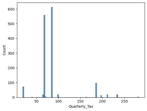

I am not sure how to accurately read the tax issues, since it is not in my area of expertise. But I am also sure that tax is a strong factor to choose and value a car. While being skeptic about this column, I’ll consider it once again in the further investigation below.

3.1.17 Weight

(Weight in Kilograms)

df.Weight.describe()

count    1436.00000
mean     1072.45961
std        52.64112
min      1000.00000
25%      1040.00000
50%      1070.00000
75%      1085.00000
max      1615.00000
Name: Weight, dtype: float64

Standard deviation is not high, it means data points are close to the mean. Let’s check the plot too.

sns.histplot(df["Weight"])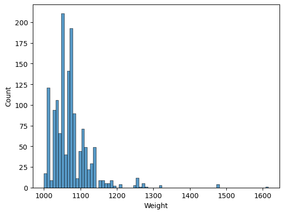

Most of us won’t talk about how much our cars weight, unless its a truck or a heavy-duty vehicle. So it was not the first thing that I think of when I choose a car, but the size and the engine volume directly effects the weight of a car. The above plot also shows varied amounts of weights, so it could be wise to consider this as well.

3.1.18 Mfr_Guarantee

Within Manufacturer’s Guarantee period (Yes=1, No=0)

df["Mfr_Guarantee"].value_counts()

0    848
1    588
Name: Mfr_Guarantee, dtype: int64

Similar to the tax-issues, the insurance & guarantee are the topics that needs deep understanding, because there are other factors than the car itself. However above digits show that there are good amount of cars that are within manufacturer’s guarantee. It can be wise to investigate this, so I’ll come to this one in further investigation again.

3.1.19 BOVAG_Guarantee

BOVAG (Dutch dealer network) Guarantee (Yes=1, No=0)

df["BOVAG_Guarantee"].value_counts()

1    1286
0     150
Name: BOVAG_Guarantee, dtype: int64

It looks like this dealer provides guarantee for most of the cars. I am not a sales-person but this seems a standard offer for most of the dealers. Again, the distribution is not varied, it doesn’t seem to help my problem statement.

3.1.20 Guarantee_Period

(Guarantee period in months)

df.Guarantee_Period.describe()

count    1436.000000
mean        3.815460
std         3.011025
min         3.000000
25%         3.000000
50%         3.000000
75%         3.000000
max        36.000000
Name: Guarantee_Period, dtype: float64

df["Guarantee_Period"].value_counts()

3     1274
6       77
12      73
24       4
36       4
18       1
13       1
20       1
28       1
Name: Guarantee_Period, dtype: int64

This shows that most of the guarantee are only for three months. This may be reflecting the dealer’s ‘standard’ offer, as I stated above. But let’s check this one too.

dealers_guar = df[(df['BOVAG_Guarantee'] == 1) & (df['Guarantee_Period'] == 3)]
len(dealers_guar)

1193

As we can see only less than 100 cars (out of those in the 3-months-guarantee-period) are not under the dealer’s offer. Since these two columns are highly related to each other and come with a dominant value each, I’ll omit them in my equation.

3.1.21 ABS

Anti-Lock Brake System (Yes=1, No=0)

df["ABS"].value_counts()

1    1168
0     268
Name: ABS, dtype: int64

A good amount of Corollas were equipped with ABS even in 2004. While the distribution is not promising, I anyway want to consider this column in my model just to check the safety measures too.

3.1.22 Airbag_1

Driver Airbag (Yes=1, No=0)

df["Airbag_1"].value_counts()

1    1394
0      42
Name: Airbag_1, dtype: int64

3.1.23 Airbag_2

Passenger Airbag (Yes=1, No=0)

df["Airbag_2"].value_counts()

1    1038
0     398
Name: Airbag_2, dtype: int64

It looks like that the airbags were already standard for driver but not for passengers. The second one can be considered with ABS together for safety choices.

3.1.24 Airco

Air conditioning (Yes=1, No=0)

df["Airco"].value_counts()

1    730
0    706
Name: Airco, dtype: int64

Almost half of the cars had air conditioning. This is a good spread of data, so I’ll put this one in the bucket as well.

3.1.25 Automatic_airco

Automatic Airconditioning (Yes=1, No=0)

df["Automatic_airco"].value_counts()

0    1355
1      81
Name: Automatic_airco, dtype: int64

Looks like only 81 out of those 730 cars airco are automatic, but I’ll check the consistency of the dataset anyway.

airco_proof = df[(df['Airco'] == 0) & (df['Automatic_airco'] == 1)]
len(airco_proof)

0

It looks cool. Let’s continue with Airco only.

3.1.26 Boardcomputer

Board computer (Yes=1, No=0)

df["Boardcomputer"].value_counts()

0    1013
1     423
Name: Boardcomputer, dtype: int64

I guess Board computer refers to the driver’s front panel which displays informations (such as fuel consumption, mileage, etc.), rather than the media screen in the middle of the front seats. But since they might be related to each other, I’ll call this column together with other three below (CD Player, Radio and Radio Cassette) as MMDs (multi-media display). As I explained at the beginning (2.2 Summary of my Initial Analysis) about the issues with the ‘radio’ values in my initial analysis, probably I’ll choose one (or max two) of these columns to be considered.

3.1.27 CD_Player

CD Player (Yes=1, No=0)

df["CD_Player"].value_counts()

0    1122
1     314
Name: CD_Player, dtype: int64

As stated above, this one goes into the MMD section for now.

3.1.28 Central_Lock

Central Lock (Yes=1, No=0)

df["Central_Lock"].value_counts()

1    833
0    603
Name: Central_Lock, dtype: int64

Central lock and the powered windows (below) both have a good distribution to be considered.

3.1.29 Powered_Windows

Powered Windows (Yes=1, No=0)

df["Powered_Windows"].value_counts()

1    807
0    629
Name: Powered_Windows, dtype: int64

3.1.30 Power_Steering

Power Steering (Yes=1, No=0)

df["Power_Steering"].value_counts()

1    1404
0      32
Name: Power_Steering, dtype: int64

Again, it seems that having a power steering is a default feauture already. I won’t put it into the equation.

3.1.31 Radio

Radio (Yes=1, No=0)

df["Radio"].value_counts()

0    1226
1     210
Name: Radio, dtype: int64

Goes into the MMD basket.

3.1.32 Mistlamps

Mist lamps (Yes=1, No=0)

df["Mistlamps"].value_counts()

0    1067
1     369
Name: Mistlamps, dtype: int64

Around a quarter of cars have mist lamps. Let’s consider them too.

3.1.33 Sport_Model

Sport Model (Yes=1, No=0)

df["Sport_Model"].value_counts()

0    1005
1     431
Name: Sport_Model, dtype: int64

Comparing to the other engine-related values like gear or volume (cc), this one seemed to me more abstract. Also the domain-knowledge plays a good role here: What is a sport model for this particular brand and model? It can be upgrade for the engine or for the outlook or for both. In my experience, in most cases it indicates some additions to the outer look of the car. So it is an effort to make the car ‘look’ like sportive, rather than ‘act’ like so. But my experience is not important, this specific car/model is essential here.

With this ambiguity I tend not to consider this deeply. But I’ll anyway investigate this in further steps below, because a good amount of cars come with sport model as the above digits reflect.

3.1.34 Backseat_Divider

Backseat Divider (Yes=1, No=0)

df["Backseat_Divider"].value_counts()

1    1106
0     330
Name: Backseat_Divider, dtype: int64

A fun fact: For couple of times I was reading this as ‘backseat driver’ and was thinking how interesting and cool this dataset was.

But unfurtunately, this is the same old, boring thing, called a divider. Probably it is the armrest (cupholder) in the middle of the backseats, but it can also mean that the backseats are foldable. I don’t know, and again I don’t want to guess also. Obviously such things cost money but I am not sure the overall effect on the entire car price or how it can effect one while choosing an older car. Yet, let’s keep it for further study anyway.

3.1.35 Metallic_Rim

Metallic Rim (Yes=1, No=0)

df["Metallic_Rim"].value_counts()

0    1142
1     294
Name: Metallic_Rim, dtype: int64

I have similar concerns for this one too as I stated above. Not sure how this can effect the price of an older car but almost 300 cars have metallic rims, so let’s keep them in the basket until further investigation.

3.1.36 Radio_cassette

Radio Cassette (Yes=1, No=0)

df["Radio_cassette"].value_counts()

0    1227
1     209
Name: Radio_cassette, dtype: int64

This one is the last column of the above-stated MMDs and it’s very close to the results for ‘Radio’, which only 210 cars have. Let’s check how many cars have both.

radio_gaga = df[(df['Radio'] == 1) & (df['Radio_cassette'] == 1)]
len(radio_gaga)

208

Looks like they are representing same set of things (radio + cassette player). So putting them in the same basket (multi-media displays) doesn’t sound as a bad idea.

Though, I understand that 2 cars having only radio without cassette player, but I don’t understand the one car that has cassette player but without a radio. That is odd. Maybe that one’s radio was broken, I don’t know. If so, then I have to put one side note here:

💡 For every boolean value, how can we be sure that they all value equally? How can we calculate those nuances within each variable? Or should we at all?

3.1.37 Parking_Assistant

Parking Assistant System (Yes=1, No=0)

df["Parking_Assistant"].value_counts()

0    1432
1       4
Name: Parking_Assistant, dtype: int64

It looks like back then parking assistant was in the luxury zone, at least for these Corollas. It wouldn’t give us much to add them in the equation.

(In fact, a lot of datasets in the web, that are titled Corolla dataset, don’t have this column at all. They were dropped as default.)

3.1.37 Tow_Bar

Tow Bar (Yes=1, No=0)

df["Tow_Bar"].value_counts()

0    1037
1     399
Name: Tow_Bar, dtype: int64

For me, the most interesting column is this tow bar. My initial analysis which revealed that tow bar’s negative effect on the price made me go that much deep into this dataset once again. It is definetely in my equation, more reasoning will come after.

3.1.38 The Summary of the Basic EDA

Ok, that was a long journey. I need a summary here. In the table below, strikethrough names represent eliminated columns, bold ones to be considered as independent variables (will be double checked with further EDA anyway) and italic ones to be investigated further.

(Spoiler Alert: This won’t be the final list.)

Id	Doors	Boardcomputer
Model	Cylinders	CD_Player
Price	Gears	Central_Lock
Age	Quarterly_Tax	Powered_Windows
Mfg_Month	Weight	Power_Steering
Mfg_Year	Mfr_Guarantee	Radio
KM	BOVAG_Guarantee	Mistlamps
Fuel_Type	Guarantee_Period	Sport_Model
HP	ABS	Backseat_Divider
Met_Color	Airbag_1	Metallic_Rim
Color	Airbag_2	Radio_cassette
Automatic	Airco	Parking_Assistant
CC	Automatic_airco	Tow_Bar

3.2 Further EDA

On this second step, I’ll check the relationships of the columns between each other and perform one more elimination phase.

3.2.1 Color

Before I go deep into a correlation matrix, let’s get the colors done first. Again, I won’t integrate a variable such as color into this MVA equation. But I anyway want to examine how cars’ colors act on the price.

With that many color options, histogram looks a bit messy, so I’ll try KDE (kernel density estimation) instead.

palette ={"Grey": 'grey', "Blue": 'blue', "Red": 'red', "Green": 'green', "Black": 'black', "Silver": 'silver', "White": 'white', "Violet": 'violet', "Yellow": 'yellow', "Beige": 'beige',}
sns.displot(df, x="Price", hue="Color", kind="kde", multiple="stack", palette=palette)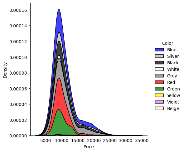

These results are interesting, let’s remember how the colors were distributed.

df["Color"].value_counts()

Grey      301
Blue      283
Red       278
Green     220
Black     191
Silver    122
White      31
Violet      4
Yellow      3
Beige       3
Name: Color, dtype: int64

Looks like blue, silver and black ones are the most popular ones. The most frequent color grey comes even after white. Maybe my comment on white color (at the beginning of the study: 3.1.10 Color) fits here as well. There are only 31 of them, yet they have a higher density here.

💡 Another point of view: Maybe white car owners don’t want to trade their cars, and keep them to themselves. Who knows?

For the moment, I’ll stop here with the ‘color’ column and I won’t consider them to serve my problem statement. These color options may be studied deeper in another analysis.

3.2.2 Correlation Matrix

Let’s check the correlation matrix without the eliminated columns.

plt.figure(figsize=(16, 14))
df_filtered = df.filter(['Age', 'KM', 'HP', 'Met_Color', 'CC', 'Doors', 'Quarterly_Tax', 'Weight', 'Mfr_Guarantee', 'ABS', 'Airbag_2', 'Airco', 'Boardcomputer', 'CD_Player', 'Central_Lock', 'Powered_Windows', 'Radio', 'Mistlamps', 'Sport_Model', 'Backseat_Divider', 'Metallic_Rim', 'Radio_cassette', 'Tow_Bar', 'Price'], axis=1)

corr = df_filtered.corr()

sns.heatmap(corr, annot=True, cmap='coolwarm', square=True)
plt.title('Correlation Matrix')
plt.show()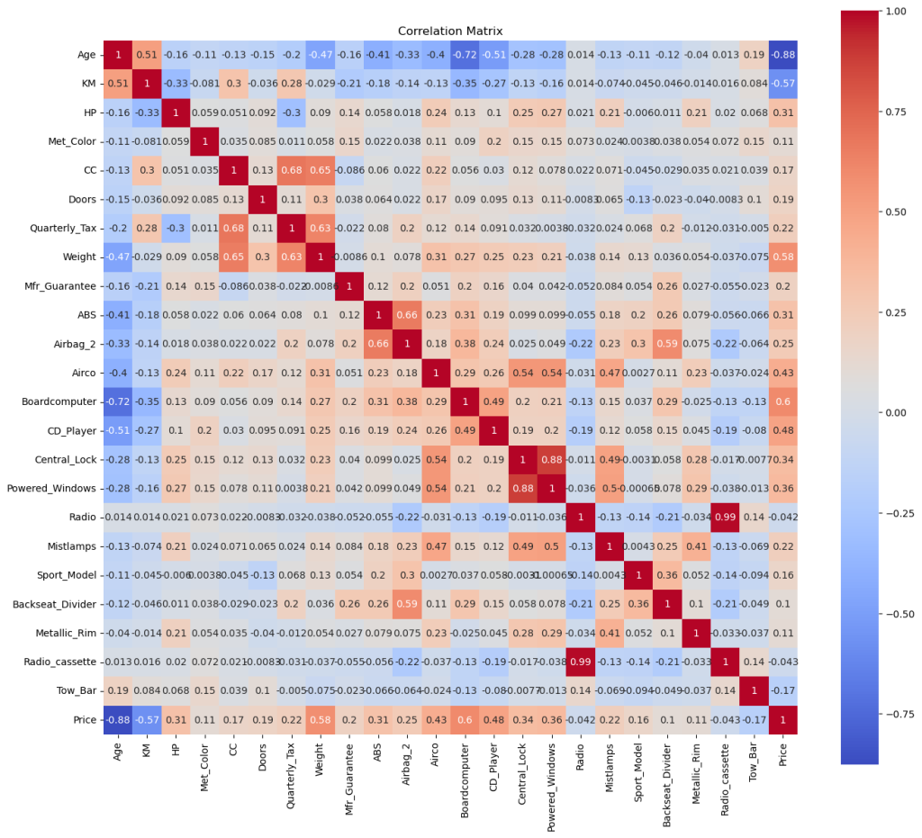

Let me continue with my notes by clustering the related features together:

3.2.3 Condition

Age and KM have the strongest negative correlation between them and the price. I’ll keep them for sure.

3.2.4 Characteristics

We don’t have fuel consumption, but we have HP and CC. So they can be considered for the engine. Doors and Weight on the other side can be considered for the size of the car. I was not sure about the weight, but it has a strong positive relation with the price. They are in.

3.2.5 Interior & MMDs

As I mentioned earlier Radio and Radio Cassette has a strong relation with each other, though their effect on price is low and negative. My counter argument (that people’s expactations for a better system) might be true, considering the strong correlation of Board Computer and CD Player. Board Computer could be enough alone, but let’s keep them both in, while taking the radios out. / Aircondition also has a strong relation, so it’s still in.

3.2.6 Features

Central Lock and Powered Windows have one of the strongest relationship between each other, which makes sense. Mostly they are connected to the same system. As you may noticed in some cars, holding longer to the lock key also rolls up the windows to close them. For the simplicity, we can keep only one of them. Say, the Powered Windows with a slightly higher correlation between it and the price. / Tow Bar, having the thirdest strongest negative correlation will be definetely in the equation and Mistlamp too is still in.

3.2.7 Exterior & Sport Model

I was thinking the Sport Models are offering some upgrades on exterior. But the matrix shows very weak relations between the sport model and the metallic rim, metallic color and also mist lamps (those are the only features I can think of as the exterior). However, the correlations between sport model and Backseat Divider, Passenger Airbag and ABS are stronger. Maybe after all, having a sport model (of these Corollas) means to have something more inside the car. Considering the weak correlation of Backseat Divider, I’ll continue with the Sport Model only (not sure though, because its correlation is also not strong with 0.16), while eliminating the divider. But let’s try to back this one up with the data itself:

df["Sport_Model"].value_counts()

0    1005
1     431
Name: Sport_Model, dtype: int64

sport_or_not = df[(df['Sport_Model'] == 1) & (df['Backseat_Divider'] == 1)]
len(sport_or_not)

431

This shows that all sport models comes with the backseat dividers. Let’s continue with the decision above. But since this sport model seems to be not related to the exterior, I’d still like to consider some outlook features. Despite the weak correlation of Metallic Rim and Metallic Color (both 0.11), I’ll give them a try.

3.2.8 Safety

ABS and Passenger Airbag‘s correlations are promising, I’ll keep them into the equation and it’s also good to have something about safety.

3.2.9 Others

I’ll eliminate the Quarter Tax, because unlike the other columns, it is affected by the price itself, not the other way around. / Although I am not quite sure about the guarantee, I’ll consider Manufacturer’s Guarantee as well. It has not so weak correlation and for most of us it is an important factor, especially when it comes to the older cars. But first I need to be sure that we have enough old cars within such guarantee.

sns.histplot(df, x="Age", hue="Mfr_Guarantee", element="step")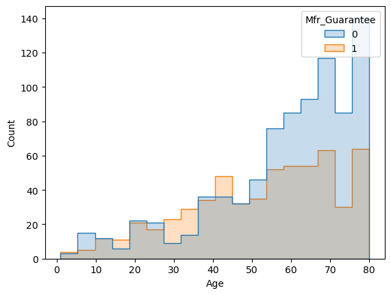

Despite the fact that only around one-third of the older cars are under the guarantee, this is still not a bad distribution. Let’s check the counts as well.

guar_for_old = df[(df['Mfr_Guarantee'] == 1) & (df['Age'] >= 60)]
len(guar_for_old)

255

len(guar_for_old) / df["Mfr_Guarantee"].sum()

0.4336734693877551

Among older cars 255 of them have guarantee and they are around 43% of the whole cars that are under such guarantee. This digits are not bad, so I’ll stick with my decision.

3.2.10 The Summary of the Further EDA

Let’s replot the correlation matrix after the second elimination, which will serve as a summary as well. This time I’ll keep the order of those clusters above.

plt.figure(figsize=(14, 12))
df_study = df.filter(['Age', 'KM', 'HP', 'CC', 'Doors', 'Weight', 'Boardcomputer', 'CD_Player', 'Airco', 'Powered_Windows', 'Tow_Bar', 'Mistlamps', 'Sport_Model', 'Metallic_Rim', 'Met_Color', 'ABS', 'Airbag_2', 'Mfr_Guarantee', 'Price'], axis=1)

corr_study = df_study.corr()

sns.heatmap(corr_study, annot=True, cmap='coolwarm', square=True)
plt.title('Correlation Matrix')
plt.show()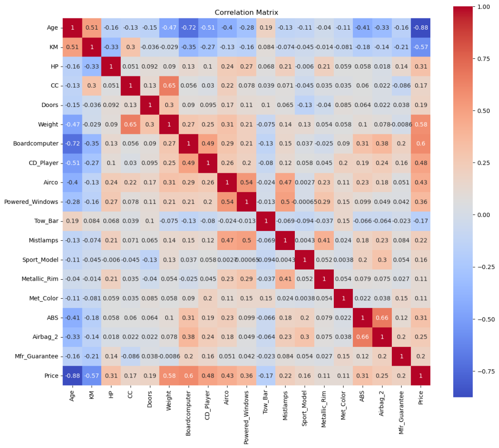

3.3 A Thousand Hidden Steps

People from the UX Design field are very well aware of the iterative structure of their work. This goes here as well. I had to come back and go forward countless times and this exact place was the peak point of those movements. I had to try a huge amount of sets (of variables) to come up with the best fitted combination to this particular model. That’s why my final set of independent variables became different than stated above. For the sake of the simplicity of the flow, I’ll just list the final variables below. At the end, I’ll come back to this ‘hidden steps’ and try my best to provide some feedback on this final elimination phase.

3.3.1 Final Variables

• Age
• KM
• HP
• Automatic
• Doors
• Mfr_Guarantee
• Airco
• CD_Player
• Powered_Windows
• Mistlamps
• Sport_Model
• Metallic_Rim
• Tow_Bar

4 Linear Regression

import sklearn
from sklearn import linear_model

4.1 Remembering the Initial Analysis

Before I jump into the final variables, I’d like to re-assign the ones from the very first analysis. As I explained at the beginning (2.2 Summary of my Initial Analysis) this time Age and KM will be added too, just to check the effects when they are into the equation. Remember, they were carrying the strongest negative correlation to the price.

y= df['Price'].values
X_init= df[['Age', 'KM', 'HP', 'Automatic', 'Doors', 'Airco', 'Powered_Windows', 'Radio', 'Tow_Bar']].values

regr_init = linear_model.LinearRegression() 
regr_init.fit(X_init, y)

# Getting the coefficiencies with a formatter to better read.
np.set_printoptions(formatter={'float_kind':'{:.2f}'.format})

# Rounding to two decimal points.
print(np.around(regr_init.coef_,2))

[-145.95 -0.01 30.84 756.35 186.71 261.61 473.17 -243.02 -243.04]

Let me put the results into a table for a better readability. First columns show the above digits, the next one reflects the initial ones. As it can be seen, the changes can be strong.

|-------------|-------------|-----------|
| age         |     -145.95 |         X |  
| km          |       -0.01 |         X |
| hp          |       30.84 |     51.65 | 
| automatic   |      756.35 |    727.40 | 
| doors       |      186.71 |    473.05 | 
| airco       |      261.61 |   2045.85 | 
| pwr windows |      473.17 |     954.6 | 
| radio       |     -243.02 |    -39.73 | 
| tow bar     |     -243.04 |   -1548.8 |

Ok, maybe this is obvious for a data scientist but for someone like me at the entry-level, this was one of those moments where I realized the importance of choosing the ‘right’ variables, deciding the ‘accurate’ models/methods and the relationship between these two. This is where I got lost in those hidden steps that I mentioned above. (I’ll come back to this again.)

4.2 Assigning the Variables

Here I am setting the independent variables for the whole set.

y= df['Price'].values
X_study= df[['Age', 'KM', 'HP', 'Automatic', 'Doors', 'Mfr_Guarantee', 'Airco', 'CD_Player', 'Powered_Windows', 'Mistlamps', 'Sport_Model', 'Metallic_Rim', 'Tow_Bar']].values

regr_study = linear_model.LinearRegression() 
regr_study.fit(X_study, y)

print(np.around(regr_study.coef_,2))

[-141.84 -0.01 28.97 747.43 234.85 105.66 159.77 251.05 346.62 366.15
 633.44 136.67 -201.59]

4.2.1 Linear Model for Older and Newer Cars

Here I am doing the same for the older (5 or more years) and -this time also- for the newer (less than 5 years) cars, by hoping to have deeper insights.

older_cars = df[(df.Age >= 60)]
newer_cars = df[(df.Age < 60)]

y= older_cars['Price'].values
X_older= older_cars[['Age', 'KM', 'HP', 'Automatic', 'Doors', 'Mfr_Guarantee', 'Airco', 'CD_Player', 'Powered_Windows', 'Mistlamps', 'Sport_Model', 'Metallic_Rim', 'Tow_Bar']].values

regr_older = linear_model.LinearRegression() 
regr_older.fit(X_older, y)

print(np.around(regr_older.coef_,2))

[-82.64 -0.01 2.45 536.67 199.53 275.87 304.95 96.71 261.91 122.65 -48.28
 96.70 -207.86]

y= newer_cars['Price'].values
X_newer= newer_cars[['Age', 'KM', 'HP', 'Automatic', 'Doors', 'Mfr_Guarantee', 'Airco', 'CD_Player', 'Powered_Windows', 'Mistlamps', 'Sport_Model', 'Metallic_Rim', 'Tow_Bar']].values

regr_newer = linear_model.LinearRegression() 
regr_newer.fit(X_newer, y)

print(np.around(regr_newer.coef_,2))

[-188.08 -0.01 42.31 656.38 216.53 122.24 296.26 90.35 97.82 774.85 723.78
 281.02 16.83]

Before I put all these digits into a table, I’ll get the average price for all mentioned age groups too. Because comparing the results alone wouldn’t reflect their proportions within the groups.

avg_all = df['Price'].mean()
avg_older = older_cars['Price'].mean()
avg_newer = newer_cars['Price'].mean()

print(f"Average price for all cars: {avg_all:.2f} €")
print(f"Average price for older cars: {avg_older:.2f} €")
print(f"Average price for newer cars: {avg_newer:.2f} €")

Average price for all cars: 10730.82 €
Average price for older cars: 8586.91 €
Average price for newer cars: 13101.07 €

5 Results

All results are collected below. First two columns (after the names) represents the digits for all cars, the middle two are for older cars (my target as stated in the problem statement), and the last two shows digits for cars that are less than 5 years old, just to read the results in a wider perspective.

Let’s inspect them all one by one. (And when I say ‘car’, I mean a ‘Toyota Corolla’ that is within this particular dataset.)

	all	10730.82	older	8586.91	newer	13101.07
Age	-141.84	-1.32%	-82.64	-0.96%	-188.08	-1.44%
KM	-0.01		-0.01		-0.01
HP	28.97	0.27%	2.45	0.03%	42.31	0.32%
Automatic	747.43	6.97%	536.67	6.25%	656.38	5.01%
Doors	234.85	2.19%	199.53	2.32%	216.53	1.65%
Mfr_Guarantee	105.66	0.98%	275.87	3.21%	122.24	0.93%
Airco	159.77	1.49%	304.95	3.55%	296.26	2.26%
CD_Player	251.05	2.34%	96.71	1.13%	90.35	0.69%
Powered_Windows	346.62	3.23%	261.91	3.05%	97.82	0.75%
Mistlamps	366.15	3.41%	122.65	1.43%	774.85	5.91%
Sport_Model	633.44	5.90%	-48.28	-0.56%	723.78	5.52%
Metallic_Rim	136.67	1.27%	96.7	1.13%	281.02	2.15%
Tow_Bar	-201.59	-1.88%	-207.86	-2.42%	16.83	0.13%

5.1 Age

These results look like the proof of that saying “Your car started to lose the value the moment you bought it.” The effect gets weaker with more than 5 years old cars, but it is still effecting the price of the car negativetely. We might have deeper understanding if we had cars -say- more than 10 years old too. Then we could check the effects after a certain age as well.

5.2 KM

This is the only variable that had the same effect on each age-group. No matter how old your car is, mileage ‘damages’ the value more or less the same. Though these same results made me question one more thing:

If we check the digits for all cars, we can say that a car getting-one-month-old costs us around 140 Euro. But to lose 100 Euro we need to drive 10k km, according to these digits. So driving 14k km ‘damages’ the value equally as the car gets just 1-month old, which is not logical at all.

When I try other set of variables (remember those hidden steps), KM always get me either -0.01 or -0.02. Even if I’ll calculate with the later one, driving 7k km, imho*, should costs us more than getting-a-month-older car.

💡 I can think of two things: There might be some other dynamics that this model could not present accurately. Or, the car dealers are really harsh when it comes to evaluate second hand cars and they use the age of an car as one of their strongest arguments to ‘price cut’.

* It's not just my opinion, it's the fact:
- According to the Enerdata, the average kilometers per a driver in Europe per year was around 13k in 2004. This dropped down to around 11.3k in 2019.[1]
- According to the Federal Highway Administration, the average annual miles per a driver in US in 2000 was around 13.5k (~21.7k km).[2] They also reported that, on average, VMT (Vehicle Miles Traveled) rose by 3.3 percent per year from 1929–2014.[3]
- According to Tuik (Turkish Statistical Institute), the average annual kilometers per a driver in Turkiye in 2020 was around 14k.[4]

5.3 HP

	all	10730.82	older	8586.91	newer	13101.07
HP	28.97	0.27%	2.45	0.03%	42.31	0.32%

It seems that having a ‘strong’ engine does not help you to sell your older Corolla. Comparing to the overall and also the newer cars, HP loses its value around 90%.

5.4 Automatic

	all	10730.82	older	8586.91	newer	13101.07
Automatic	747.43	6.97%	536.67	6.25%	656.38	5.01%

No matter how old your car is, having an automatic gear is a valuable thing. I am aware that I need to be careful here, because we don’t have much cars with an automatic gear in this dataset. But as I’ll explain below (6.3 Automatic Gear) the reflective distribution helps me to say so. Besides, considering that this dataset is from 2004 and how automatic cars are popular now,
💡 maybe we can safely claim that there was a demand towards this direction even that time.

5.5 Doors

	all	10730.82	older	8586.91	newer	13101.07
Doors	234.85	2.19%	199.53	2.32%	216.53	1.65%

If we can read the number of doors as an indicator for the size of the car, we can also tell by checking this result that the size of the car is an important factor for all ages. In fact, if we check the percentages (to the mean of the price) its effects gets stronger on older cars.

💡 Maybe we can claim that asking for a bigger car is more common among cars that are older than 5 years.

5.6 Mfr_Guarantee

	all	10730.82	older	8586.91	newer	13101.07
Mfr_Guarantee	105.66	0.98%	275.87	3.21%	122.24	0.93%

This was a hypothesis that I wanted to test and the results proofed it. No surprize here, if your car is under manufacturer’s guarantee, you can value it higher. It is even more important for the older cars.

5.7 Airco

	all	10730.82	older	8586.91	newer	13101.07
Airco	159.77	1.49%	304.95	3.55%	296.26	2.26%

As it was with the guarantee, I was expecting that having an air conditioning would mean more for older cars. I am glad that these results reflects this, unlike in my initial analysis. In that study, despite the positive effect on the price, it was less effective compared to the whole cars. Again, I think this was caused by the variable choices.

5.8 CD Player & Powered Windows

	all	10730.82	older	8586.91	newer	13101.07
CD_Player	251.05	2.34%	96.71	1.13%	90.35	0.69%
Powered_Windows	346.62	3.23%	261.91	3.05%	97.82	0.75%

I was thinking that having powered windows and CD player would be more important when your car is old, like as having an air conditioning. For these, the effect gets weaker compared to all cars. But having a second look at the newer cars, the importance is underlined for older cars.
💡 We can also claim that people who are buying newer cars, already expect to have powered windows (and CD Player) as default, so it’s effect is less strong compared to the older ones.

5.9 Mist Lamps & Metallic Rim

	all	10730.82	older	8586.91	newer	13101.07
Mistlamps	366.15	3.41%	122.65	1.43%	774.85	5.91%
Metallic_Rim	136.67	1.27%	96.7	1.13%	281.02	2.15%

Mist lamps and Metallic rims were not in my main focus, simply because I was thinking that they won’t serve the problem statement. In fact, the correlation matrix also showed not so strong digits (0.22 and 0.11 respectively) for their relations to the price. I anyway wanted to examine some features about the outlook of the car. We can tell that both add value to your car, but loses their effects when your car is getting older than 5 years.

However, an additional look to the correlation matrix reveals some other things. Check their strongest relations with some other features below.

Mistlamps > Powered Windows (0.59) / Airco (0.47) / Metallic Rim (0.41)
Metallic Rim > Mistlamps (0.41) / Powered Windows (0.29) / Airco (0.23)

These numbers show how these are related to each other. This kind of further investigation did shape this analysis much and below you will see other samples.

5.10 Sport Model

	all	10730.82	older	8586.91	newer	13101.07
Sport_Model	633.44	5.90%	-48.28	-0.56%	723.78	5.52%

You may remember how I revealed the relationship between the Sport Model and the Backseat Divider (3.2.7 Exterior & Sport Model). To understand its negative effect on older cars, let’s check the strongest relations as we did above. I’ll add Backseat Divider as well for a wider perspective.

Sport Model > Backseat Divider (0.36) / Airbag_2 (0.3) / ABS (0.2)
Backseat Divider > Airbag_2 (0.59) / Sport Model (0.36) / Boardcomputer (0.29) / ABS (0.26) / Mistlamp (0.25)

So Sport Model and all these kind of features may represent some additional packages that car producers offer. And checking the newer (and all) cars results above, we can tell that they are somehow indicating being new. Investigations below will support this view too.

5.11 Tow Bar

	all	10730.82	older	8586.91	newer	13101.07
Tow_Bar	-201.59	-1.88%	-207.86	-2.42%	16.83	0.13%

This is the most fun part of this analysis for me. After all, the strong but negative effect (on price) of having a tow bar brought me up here. Ok, some other things as well! But unlike other ‘surprizing’ results, tow bar indeed had a negative correlation between the price as the matrix presented. I have to admit that I was not aware of this while working on the initial analysis. This made me question my (and also the instructors) expectations and interpretations (that I mentioned at the beginning in 2.2 Summary of my Initial Analysis).

After spending some time in internet and reading articles titled like “What Are the Dangers of Buying a Car With a Towbar Already Fitted?” and forum posts asking questions like “Towbar take it off or leave it on when trading in?” or “Used cars with tow bars – more risky to buy?“, I’ve come to a conclusion that having a towbar really can decrease the price of a car. Mainly because the dealers tendency to read them as a sign of a car being ‘used roughly’.

Again, it looks like that the importance of domain-knowledge plays an essential role* here. But even so, I need to find some concrete proof within this database to support this thesis. Because even if this is a thing, it might not be a case for our situation.

* Ok, I need one more side note here: Remember my doubt about the Boolean values?: How can they all weight the same? If a dealer checks your car's tow bar just visually and notes it as something 'bad' without further investigation, then my question gets even stronger. Having a tow bar shouldn't mean something, how-it-was-used may be. Remember that old car commercial? (this or this)

Then, I started to dig deeper into the dataset and used similar methods as stated above. Let’s first check how many older cars have tow bar.

tow_old = df[(df['Tow_Bar'] == 1) & (df['Age'] >= 60)]
len(tow_old)

253

That’s more than half of the total tow bar cars (we had 399 of them). Let’s check the whole picture.

sns.histplot(df, x="Age", hue="Tow_Bar", element="step")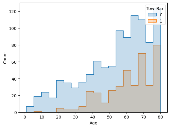

This graph shows clearly that most of the tow bars showing themselves after around 3 years (36 months) and close to 5 years it reaches a point where older cars with a tow bar did not get below that level. So apart from the concerns that were raised in those forums above, here in this particular dataset having a tow bar could mean having an old car too. If they were not coming as a default part of those Corollas, then it could really mean that the owners did ‘touch’ the car in the way that dealers evaluate negatively.

So I think I got my answer to the tow bar question! Or at least for now, I am convinced with what I got.

This brings me to those hidden steps (that I mentioned above in the section 3.3). While trying to figure out the results, I started to try tons of different set of variables to get a wider angle which made me realize the probability of such relationships as I mentioned here. So let me demonstrate some of such investigations from those hidden steps.

6 Coming back to those Hidden Steps

Here I’ll try to explain why I left some more variables out of my equation after the second round of the EDA.

6.1 Board Computer, ABS and Passenger Airbag

In all combinations of my variables these three were giving me negative results. This was unexpected, because all had positive correlation between them and the price (0.6, 0.31 and 0.25 respectively). Considering that the Board Computer had the strongest positive correlation, this became even more interesting. But the matrix also revealed a very strong but negative correlation (-0.72) between the Board Computer and the Age. We need to look at this situation closer.

sns.histplot(df, x="Age", hue="Boardcomputer", element="step")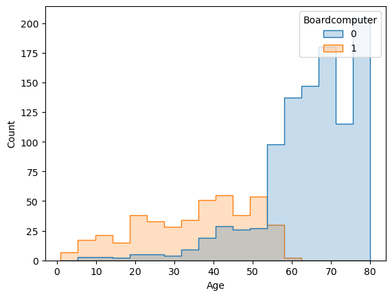

I guess this is the place where I can use that phrase: A picture is worth a thousand words. The cars that don’t have Board Computer start to rise with around 30 months old cars and after 5 years none of the cars have it. So not having a board computer -here- is a very strong indicator of being an old car. A similar pattern can be found with the ABS and the Airbag_2, but not as dramatic as this one. I believe this can be the reason of those negative results when it comes to coefficients. Or, maybe we can claim that their relationships does not fit to a linear model. / That’s why I eliminated these.

6.2 Weight and CC

I wanted to consider both Weight and Doors together to check the effects of the car size. They were giving ‘expected’ results when only one of them were in the list of the variables. However, Doors were giving negative results when the Weight were introduced in. Eliminating Weight was a better fit for this model, but considering their distributions I guess that both were not a good fit for a linear model. / Despite its positive correlation (0.17) the CC column was also not consistent. It might be caused due to the distribution again. Remember that 1600cc was dominating the column (Section 3.1.12).

6.3 Automatic Gear

You may remember that I left the Automatic gear out of my equation in the first round of EDA, because of the ‘poor’ distribution. However on all the iterations that I’ve given a try, they were consistent and positive. That’s why I double checked the situation.

sns.histplot(df, x="Age", hue="Automatic", element="step")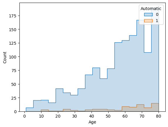

Although it is weak, the non-automatic cars distribution follows similar pattern with the automatic ones. 50 out of 80 automatic cars were over 5 years old. That’s why I kept them in the variables. Said that, I did not do the same for Automatic Air Conditioning, even though it gave very positive digits. Because only 4 out of 81 cars with automatic airco were over 5 years old.

7 Conclusion

Ok, I need an ending, right? If you followed all steps till here, I am grateful to your patience. This is my final note:

If you are a 5-or-6-years-old Corolla owner and the year is 2004 and you want to check this dealer’s offer to trade your car, here is what I can tell you based on the steps above:

7.1 Do These

✅ If the car has an automatic gear, start your bargain with it. Tell them how smoothly it works!
✅ The same goes for your cool air conditioning. (If you did change the filter, you can mention that too. But don’t forget: No data is shown above related to any filter.)
✅ While telling all of these, roll up and down your powered windows. Show them who has the power!
✅ If your car is still under the manufacturer’s guarantee, you should definetely talk about it.
☑️ If you feel the vibe is positive, add some flavors by telling about your mist lamps and metallic rims. But don’t rely on these much.

7.2 Don’t Do These

❌ If your car has a strong engine, better not brag about your horses!
❌ If your car’s sportive outlook is all about that backseat divider, don’t even mention it.
❌ Never, ever think to tell how ‘good’ your car is by reasoning it with its ability to pull heavy trailers with that tow bar. If the dealers use the tow bar as an argument for price cut, tell that you only carried your 5-years-old kid’s bicycle on that. (But again, there is no data above about any kid’s bike)

---

8 Going Forward

Takeaways

What I learned:

Working with that many variables can be hard in terms of the finding related ones. Coming up with a concrete problem statement at the very beginning of the analysis helped me to stay on track.

Said that, a good domain-knowledge is essential for every single data-related research.

No matter how sure you (and your colleagues) would be about one particular outcome, the data may (and most probably will) show something else and more.

Next Steps

If I’d have more time, I could study the followings:

---

---