Probability distribution describes the likelihood of the possible outcomes of a random event. Here we’ll study both discrete and continuous probability distributions. Let’s first talk about some basics.
Random variable represents the values for the possible outcomes of a random event.
Discrete random variable has a countable number of possible values. (~dice outcomes)
Continuous random variable takes the possible values in some range of numbers. (~height, time, temperature)
Discrete or continuous variables:
Count the number of outcomes discrete
Measure the outcome continuous
Sample space – the set of all possible values for a random variable.
Sample space for single coin toss = {Heads, Tails}
Sample space for single die roll = {1, 2, 3, 4, 5, 6}
A. Discrete probability distributions
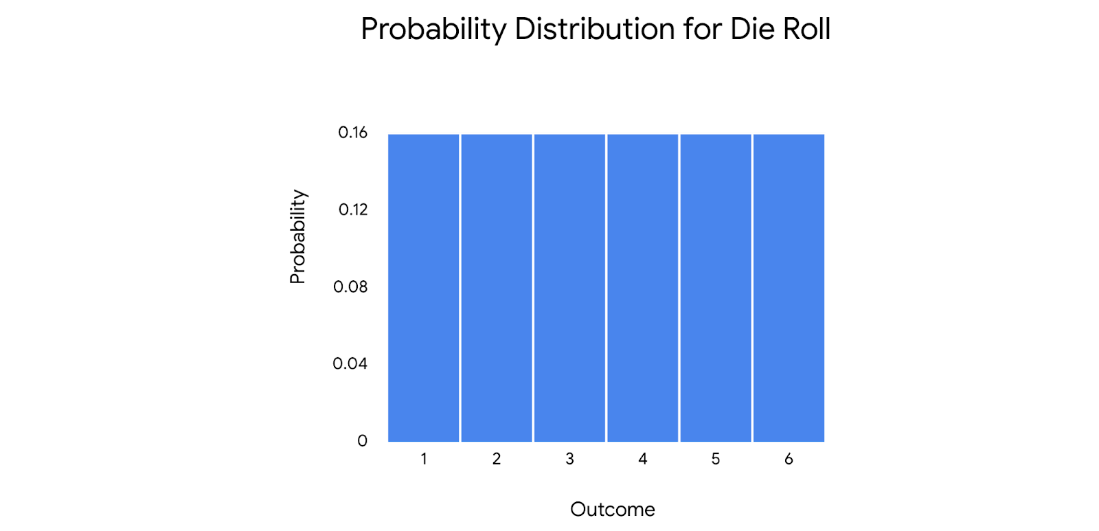
Uniform distribution
The uniform distribution describes events whose outcomes are all equally likely, or have equal probability. For example, rolling a die can result in six outcomes: 1, 2, 3, 4, 5, or 6. The probability of each outcome is the same: 1 out of 6, or about 16.7%.
The uniform distribution applies to both discrete and continuous random variables.
The binomial distribution
A discrete distribution that models the probability of events with only two possible outcomes, success or failure.
This definition assumes that
- each event is independent or does not affect the probability of the others,
- and that the probability of success is the same for each event.
Mutually exclusive – two outcomes are mutually exclusive if they cannot occur at the same time.
Data professionals use the binomial distribution to model data in
- Medicine (~a new medication generates side effects)
- Banking (~credit card transaction is fraudulent)
- Investing (~stock price rises or falls in value)
- Machine learning (to classify data: ~train an algorithm to recognize whether a digital image of an animal is or is not a cat)
Reminder: Random experiment is a process whose outcome cannot be predicted with certainty.
All random experiments have three things in common.
- The experiment can have more than one possible outcome.
- We can represent each possible outcome in advance.
- The outcome of the experiment depends on chance.
On the other hand, a binomial experiment has the following attributes.
- The experiment consists of a number of repeated trials.
- Each trial has only two possible outcomes.
- The probability of success is the same for each trial.
- Each trial is independent.
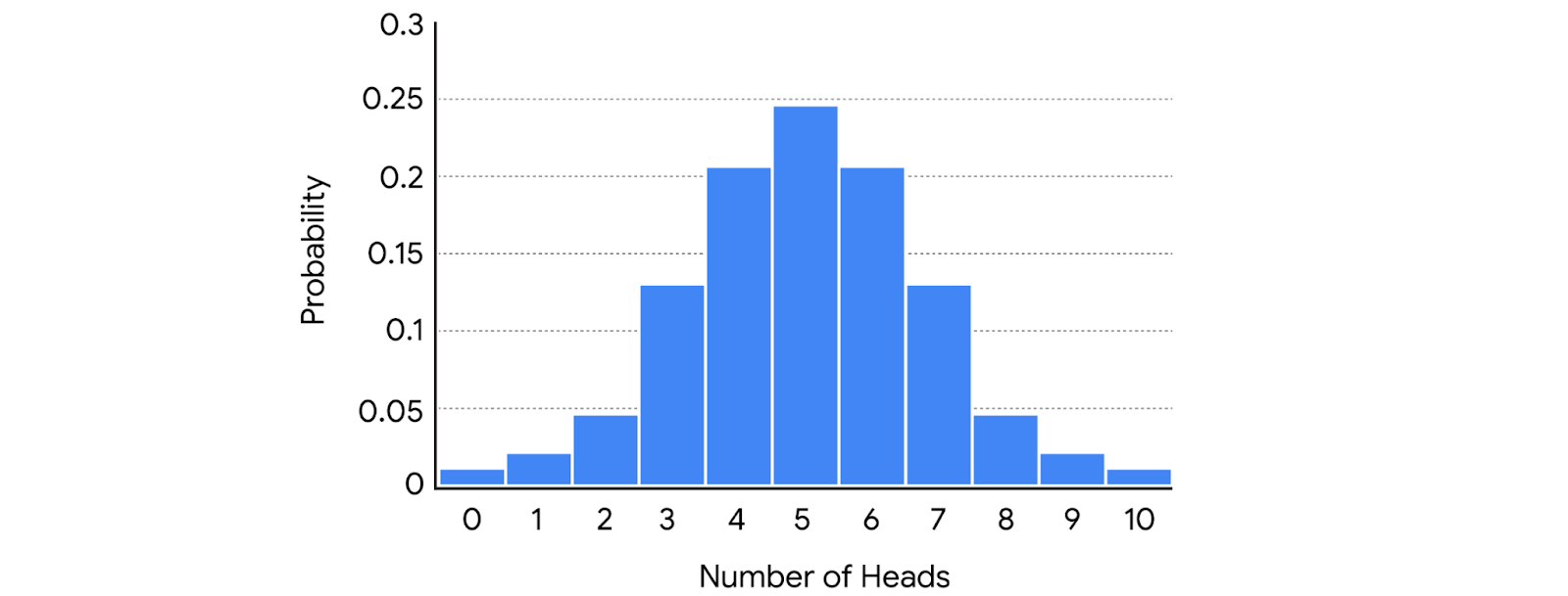
An example of a binomial experiment is tossing a coin 10 times in a row. Because it has the following features.
- The experiment consists of 10 repeated trials or coin tosses.
- Each trial has only two possible outcomes, heads or tails.
- The probability of success is the same for each trial: 50%.
- Each trial is independent: The outcome of one coin toss does not affect the outcome of any other coin toss.
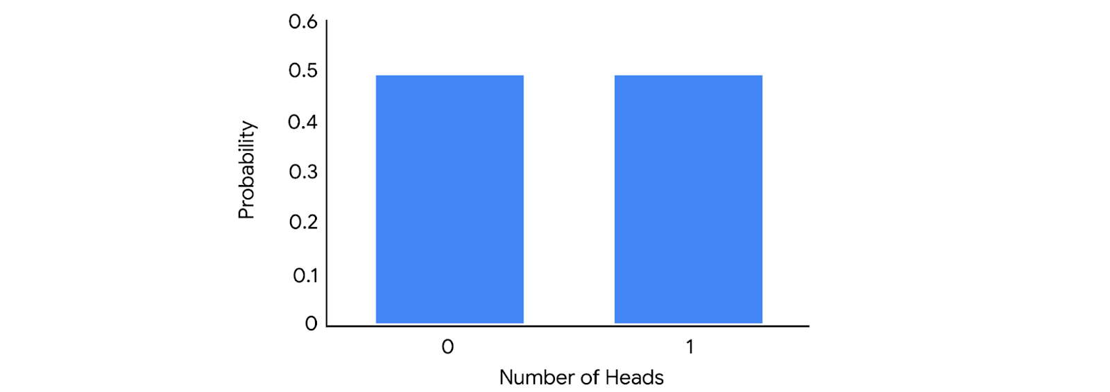
Bernoulli distribution
The Bernoulli distribution is similar to the binomial distribution as it also models events that have only two possible outcomes (success or failure). The only difference is that the Bernoulli distribution refers to only a single trial of an experiment, while the binomial refers to repeated trials. A classic example of a Bernoulli trial is a single coin toss.
The Poisson distribution
Models the probability that a certain number of events will occur during a specific time period. The Poisson distribution can also be used to represent the number of events that occur in a specific space, such as a distance, area, or volume, but here we’ll focus on time.
Data professionals use the Poisson distribution to model data such as:
- (the expected number of) calls per hour for a customer service call center,
- visitors per hour for a website,
- customers per day at a restaurant,
- severe storms per month in a city,
- Financial transactions per second at a bank.
A Poisson experiment has the following attributes;
- The number of events in the experiment can be counted.
- The mean number of events that occurred during a specific time period is known.
- Each event is independent.
A sample: Let’s imagine we have an online website where we post content. Our website averages two views per hour. We want to determine the probability that our website will receive a certain number of views in a given hour.
This sample has the following features that makes it a Poisson experiment:
- The number of events in the experiment can be counted. You can count the number of views.
- The mean number of events that occur during a specific time period is known. There is an average of two views per hour.
- Each outcome is independent. The probability of one person viewing your website does not affect the probability of another person viewing your website.
Poisson distribution formula is:
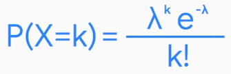
where
λ (lambda) refers to the mean number of events that occur during a specific time period
k refers to the number of events
e is a constant equal to approximately 2.71828
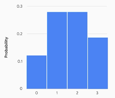
If we check the probability for 0, 1, 2, and 3 views per hour, the results will be:
P(X=0) = 0.1353
P(X=1) = 0.2707
P(X=2) = 0.2707
P(X=3) = 0.1805
We can visualize these results with histogram as below. X-axis shows the number of events (views per hour), y-axis shows the probability of occurrence.
Which one to use: Poisson vs Binomial
| Given | Want to find | Example | |
| Poisson | The average probability of an event happening for a specific time period | The probability of a certain number of events happening in that time period | The probability of getting 12 calls between 2 pm and 3 pm |
| Binomial | An exact probability of an event happening | The probability of the event happening a certain number of times in a repeated trial | The probability of getting 8 heads in 10 coin tosses |
B. Continuous probability distributions
Before we get to the specific attributes of the normal distribution, let’s discuss some general features of all continuous probability distributions. There are two types of probability functions:
- Probability Mass Functions (PMFs) represent discrete random variables
- Probability Density Functions (PDFs) represent continuous random variables
A probability function can be represented as an equation or a graph. The math involved in probability functions is beyond the scope of this post. For now, it’s important to know that the graph of a PDF appears as a curve.
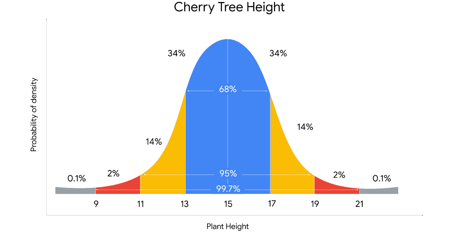
Let’s say we want to know the probability that the height of a randomly chosen cherry tree is exactly 15.1 feet. Because the height of the tree could be any decimal value in a given interval, the probability of any specific value is zero. So it only makes sense to talk about the probabilities of intervals.
The normal distribution (aka Gaussian distribution)
The Gaussian or normal distribution is a continuous probability distribution that is symmetrical on both sides of the mean and bell-shaped.
The normal distribution is the most common probability distribution in statistics because so many different kinds of data sets display a bell-shaped curve. For example, if we randomly sample 100 people we’ll discover a normal distribution curve for continuous variables, such as: height, weight, blood pressure, IQ scores, salaries, shoe size, and more.
On a normal curve the x-axis refers to the value of the variable we’re measuring and the y-axis refers to how likely we are to observe the value.
Data professionals use the normal distribution to model all kinds of different data sets in the fields of business, science, government, machine learning, and others.
All normal distributions have the following features:
- the shape is a bell curve,
- the mean is located at the center of the curve,
- the curve is symmetrical on both sides of the center,
- the total area under the curve equals 1.
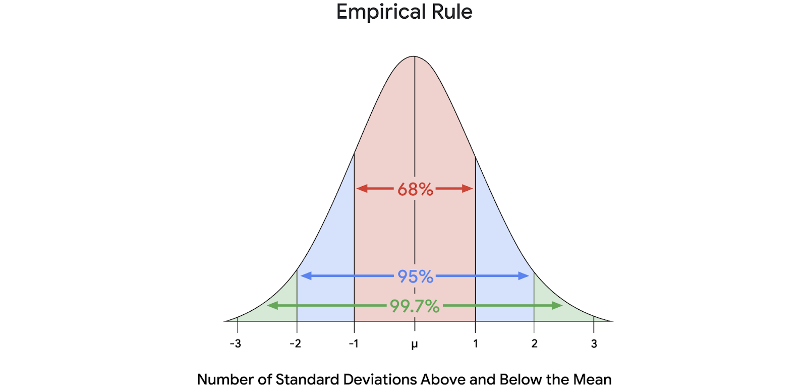
The empirical rule
It states that for a given data set with a normal distribution:
- 68 percent of values fall within one standard deviation of the mean
- 95 percent of values fall within two standard deviations of the mean
- 99.7 percent of values fall within three standard deviations of the mean
The empirical rule can give us a quick estimate of how the values in a large dataset are distributed. This saves time and helps us better understand our data.
Knowing the location of our values on a normal distribution is also useful for detecting outliers. Typically, data professionals consider values that lie more than 3 standard deviations below or above the mean to be outliers.
It’s important to identify outliers because some extreme values may be due to errors in data collection or data processing, and these false values may skew our results.
Standardize data using z-scores
Z-score is a measure of how many standard deviations below or above the population mean a data point is. In statistics, standardization is the process of putting different variables on the same scale.
Z-scores are also called standard scores because they’re based on what’s called the standard normal distribution. A standard normal distribution is just a normal distribution with a mean of 0 and a standard deviation of 1. Z-scores typically range from -3 to +3.
Standardization is useful because it lets us compare scores from different data sets that may have different units, mean values and standard deviations. Data professionals use z-scores to better understand the relationship between data values within a single dataset and between different data sets.
Data professionals often use z-scores for anomaly detection, which finds outliers in datasets. Applications of anomaly detection include:
- finding fraud in financial transactions,
- flaws in manufacturing products,
- intrusions in computer networks and more.
For example, different customer satisfaction surveys may have different rating scales. One survey could rate a product or service from 1 to 20, another from 500 to 1,500, and a third from 130 to 180.
We can use the following formula to calculate a z-score:
z = (x-μ)/σ
x refers to a single data value or raw score.
The Greek letter mu refers to population mean.
The Greek letter sigma refers to the population standard deviation.
So we can also say that Z equals the raw score or data value minus the mean divided by the standard deviation.