
My role
Data Analysis & Research
Performing a Data Analysis for Marketing Team to reveal potential growth

Timeline
May ’24
Case study, Google’s Data Analytics Cert. Prog.

Tools
R & Jupyter
Office Suite
FigJam
Tableau
OVERVIEW
The Data
The Divvy Bike, bike-sharing company, keeps records of the trips and the stations. Their dataset has observations since 2013 and here I studied the year 2023.
The Goal
Identify how annual members and casual riders use bikes differently, find why casual riders would buy a membership and suggest alternatives.
Tools
Tidyverse for basics,
Skimr and Naniar for analysis and visualization,
Tableau for visualization.
Methods
Statistics
Data Cleaning
Data Analysis
Problem Statements
Data Visualization
Data Manipulation
Research data *
I do not own the Divvy Bike dataset, and below you will find more information about it. The data has been made available to the public under this license.
* I performed this analysis only for educational purposes and to demonstrate my skills and how I approach to a dataset, that has a long-list of observations.
1 Introduction
In this case study, I’ll be acting as a Jr. data analyst in the marketing analyst team at Divvy Bikes, a bike-share company in Chicago. The director of marketing believes the company’s future success depends on maximizing the number of annual memberships.
Therefore, we want to understand how casual riders and annual members use Divvy bikes differently. From these insights, we will design a new marketing strategy to convert casual riders into annual members.
1.1 About the Company
Divvy is the bicycle sharing system in the Chicago metropolitan area, currently serving the cities of Chicago and Evanston. The system is owned by the Chicago Department of Transportation and has been operated by Lyft since 2019. As of Sept 2021, Divvy operated 16,500 bicycles and over 800 stations, covering 190 square miles.
The director of marketing believes that maximizing the number of annual members will be key to future growth. Rather than creating a marketing campaign that targets all-new customers, she believes there is a very good chance to convert casual riders into members.
1.2 The Source of the Dataset
The Divvy Bike keeps records of the trips and the related stations. The dataset has observations since 2013 and the full list can be found here. The data has been made available to the public under this license. Throughout the years the city of Chicago increased their Bikeshare Network, and a map that reflects this progress can be found here.
1.3 The Metadata
The tables have the following variables:
| variables | description |
|---|---|
| ride_id | ID attached to each trip taken |
| rideable_type | types of the bikes |
| started_at | day and time trip started, in CST |
| ended_at | day and time trip ended, in CST |
| start_station_name | name of station where trip originated |
| start_station_id | ID of station where trip originated |
| end_station_name | name of station where trip terminated |
| end_station_id | ID of station where trip terminated |
| start_lat | starting station latitude |
| start_lng | starting station longitude |
| end_lat | ending station latitude |
| end_lng | ending station longitude |
| member_casual | “Casual” is a rider who purchased a 24-Hour Pass; “Member” is a rider who purchased an Annual Membership |
1.4 Data Storage
I downloaded last years’ files (that is 2023) to track the trends throughout the year and used Kaggle’s servers to locate the dataset. Records are hold separately for each month and the column names and the data types are consistent throughout the full dataset (for all months of 2023).
2 Statement of the Business Task
The director of marketing has set a clear goal: Design marketing strategies aimed at converting casual riders into annual members. In order to do that, the marketing analyst team needs to better understand:
- how annual members and casual riders differ,
- why casual riders would buy a membership, and
- how digital media could affect their marketing tactics.
The marketing team are interested in analyzing the Divvy historical bike trip data to identify trends.
2.1 Loading the Data
library(tidyverse)

list.files(path = "../input")
Before I load all csv files and combine them, I’ll have a quick look at the first one that is for January of 2023. By this I am hoping to get a good sense of the information the datasets carry.
str(trips_2301)spc_tbl_ [190,301 × 13] (S3: spec_tbl_df/tbl_df/tbl/data.frame)
$ ride_id : chr [1:190301] "F96D5A74A3E41399" "13CB7EB698CEDB88" "BD88A2E670661CE5" "C90792D034FED968" ...
$ rideable_type : chr [1:190301] "electric_bike" "classic_bike" "electric_bike" "classic_bike" ...
$ started_at : POSIXct[1:190301], format: "2023-01-21 20:05:42" "2023-01-10 15:37:36" ...
$ ended_at : POSIXct[1:190301], format: "2023-01-21 20:16:33" "2023-01-10 15:46:05" ...
$ start_station_name: chr [1:190301] "Lincoln Ave & Fullerton Ave" "Kimbark Ave & 53rd St" "Western Ave & Lunt Ave" "Kimbark Ave & 53rd St" ...
$ start_station_id : chr [1:190301] "TA1309000058" "TA1309000037" "RP-005" "TA1309000037" ...
$ end_station_name : chr [1:190301] "Hampden Ct & Diversey Ave" "Greenwood Ave & 47th St" "Valli Produce - Evanston Plaza" "Greenwood Ave & 47th St" ...
$ end_station_id : chr [1:190301] "202480.0" "TA1308000002" "599" "TA1308000002" ...
$ start_lat : num [1:190301] 41.9 41.8 42 41.8 41.8 ...
$ start_lng : num [1:190301] -87.6 -87.6 -87.7 -87.6 -87.6 ...
$ end_lat : num [1:190301] 41.9 41.8 42 41.8 41.8 ...
$ end_lng : num [1:190301] -87.6 -87.6 -87.7 -87.6 -87.6 ...
$ member_casual : chr [1:190301] "member" "member" "casual" "member" ...
- attr(*, "spec")=
.. cols(
.. ride_id = col_character(),
.. rideable_type = col_character(),
.. started_at = col_datetime(format = ""),
.. ended_at = col_datetime(format = ""),
.. start_station_name = col_character(),
.. start_station_id = col_character(),
.. end_station_name = col_character(),
.. end_station_id = col_character(),
.. start_lat = col_double(),
.. start_lng = col_double(),
.. end_lat = col_double(),
.. end_lng = col_double(),
.. member_casual = col_character()
.. )
- attr(*, "problems")=<externalptr>
head(trips_2301)| ride_id | rideable_type | started_at | ended_at | start_station_name | start_station_id | end_station_name | end_station_id | start_lat | start_lng | end_lat | end_lng | member_casual |
|---|---|---|---|---|---|---|---|---|---|---|---|---|
| <chr> | <chr> | <dttm> | <dttm> | <chr> | <chr> | <chr> | <chr> | <dbl> | <dbl> | <dbl> | <dbl> | <chr> |
| F96D5A74A3E41399 | electric_bike | 2023-01-21 20:05:42 | 2023-01-21 20:16:33 | Lincoln Ave & Fullerton Ave | TA1309000058 | Hampden Ct & Diversey Ave | 202480.0 | 41.92407 | -87.64628 | 41.93000 | -87.64000 | member |
| 13CB7EB698CEDB88 | classic_bike | 2023-01-10 15:37:36 | 2023-01-10 15:46:05 | Kimbark Ave & 53rd St | TA1309000037 | Greenwood Ave & 47th St | TA1308000002 | 41.79957 | -87.59475 | 41.80983 | -87.59938 | member |
| BD88A2E670661CE5 | electric_bike | 2023-01-02 07:51:57 | 2023-01-02 08:05:11 | Western Ave & Lunt Ave | RP-005 | Valli Produce – Evanston Plaza | 599 | 42.00857 | -87.69048 | 42.03974 | -87.69941 | casual |
| C90792D034FED968 | classic_bike | 2023-01-22 10:52:58 | 2023-01-22 11:01:44 | Kimbark Ave & 53rd St | TA1309000037 | Greenwood Ave & 47th St | TA1308000002 | 41.79957 | -87.59475 | 41.80983 | -87.59938 | member |
| 3397017529188E8A | classic_bike | 2023-01-12 13:58:01 | 2023-01-12 14:13:20 | Kimbark Ave & 53rd St | TA1309000037 | Greenwood Ave & 47th St | TA1308000002 | 41.79957 | -87.59475 | 41.80983 | -87.59938 | member |
| 58E68156DAE3E311 | electric_bike | 2023-01-31 07:18:03 | 2023-01-31 07:21:16 | Lakeview Ave & Fullerton Pkwy | TA1309000019 | Hampden Ct & Diversey Ave | 202480.0 | 41.92607 | -87.63886 | 41.93000 | -87.64000 | member |
2.2 Checking for the Missing Values and the Duplicates
With the following code, I’ll dedect:
- Columns with missing values,
- Total number of rows with minimum one missing value,
- Count of missing values by each column,
- The duplicates if exist.
print("Columns with missing values of Jan 2023")
names(which(colSums(is.na(trips_2301)) > 0))

print("No of Rows with min. one missing value, for Jan 2023")
missing_rows_01 <- trips_2301 %>%
                    filter(!complete.cases(.))
nrow(missing_rows_01)

print("Count of missing values of Jan 2023 by column")
sapply(trips_2301, function(x) sum(is.na(x)))

print("Count of duplicated rows in Jan 2023")
sum(duplicated(trips_2301))
[1] "Columns with missing values of Jan 2023"
'start_station_name''start_station_id''end_station_name''end_station_id''end_lat''end_lng'
[1] "No of Rows with min. one missing value, for Jan 2023"
42017
[1] "Count of missing values of Jan 2023 by column"
ride_id0 rideable_type0 started_at0 ended_at0 start_station_name26721 start_station_id26721 end_station_name27840 end_station_id27840 start_lat0 start_lng0 end_lat127 end_lng127 member_casual0
[1] "Count of duplicated rows in Jan 2023"
0
2.3 Data Consistency
Before summarizing the results above, let’s first be sure about the consistency of the dataset. Below I’ll check:
- Missing values within the same group of columns listed above,
- If the names & ids and names & coordinates (lat and lng) are consistent or not.
# Checking if those missing values are matching within each group or not.

missing_start_stations <- trips_2301 %>%
                        filter((is.na(start_station_name)) & (is.na(start_station_id)))
nrow(missing_start_stations)

missing_end_stations <- trips_2301 %>%
                        filter((is.na(end_station_name)) & (is.na(end_station_id)))
nrow(missing_end_stations)

missing_end_lat_lng <- trips_2301 %>%
                        filter((is.na(end_lat)) & (is.na(end_lng)))
nrow(missing_end_lat_lng)
26721
27840
127
# Cross-checking the Name, Id and Coordinates of the Stations.

trips_2301_stations <- trips_2301 %>%
    filter((start_station_name == start_station_name & start_lat != start_lat) |
           (start_station_name == start_station_name & start_lng != start_lng) |
           (end_station_name == end_station_name & end_lat != end_lat) |
           (end_station_name == end_station_name & end_lng != end_lng) |
           (start_station_name == start_station_name & start_station_id != start_station_id) |
           (end_station_name == end_station_name & end_station_id != end_station_id))

nrow(trips_2301_stations)
0
Looks like they are consistent. Both results above repeat in all months’ datasets as a pattern. A Summary of Missing Values would be like this:
- Only the columns ‘start_station_name’ & ‘start_station_id’, ‘end_station_name’ & ‘end_station_id’ and ‘end_lat’ & ‘end_lng’ have the missing values.
- start_name & start_id, end_name & end_id, end_lat & end_lng act as groups, meaning that each column within a group have the common missing values.
- There are no duplicates.
2.3.1 Side Note to myself: Venn Diagram for Missing Values
I was trying to find a easier way to demonstrate how those missing values intersect with each other, if they do so. I wanted to see them as a venn diagram, that would help me to see their relations quickly and I wanted to have some kind of function that would give me this automatically. However I was not able to do so and it seemed that I had to hard-code the values by myself.
Just to have this process on my notes, here I am keeping that code for Venn diagram. But luckily later on further EDA phase I found another way (UpSet Table) to do this. I’ll perform that later on.
# For this I need another package.

install.packages("VennDiagram")
library(VennDiagram)
grid.newpage() # Move to new plotting page
draw.triple.venn(area1 = 26721, # Create venn diagram with three sets
area2 = 27840,
area3 = 127,
n12 = 12544,
n23 = 127,
n13 = 0,
n123 = 0,
category= c("Start Station" , "End Station" , "Lat & Lng"),
cat.pos = c(-20, 20, 180),
cat.dist = c(0.05, 0.05, 0.025),
cat.col = rep("blue", 3))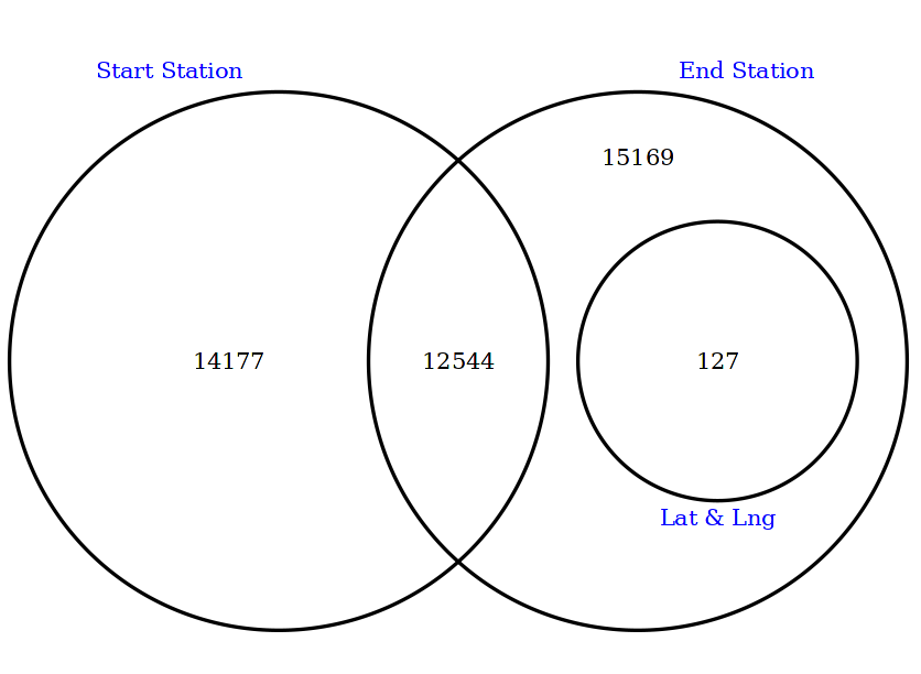
# Those digits above come from codes that reflects intersections like below:

missing_start_end <- trips_2301 %>%
                         filter((is.na(start_station_name)) & (is.na(end_station_name)))
nrow(missing_start_end)
12544
3 Basic EDA: Plotting the Raw Data
Before doing anything with the missing values I’ll get a glimpse of the raw data, to understand what’s in it as a whole. For all months separately I’ll check the distributions of the Users and the Bikes. By this, I’ll get:
- Total number of rides by users (members or casuals) per month and their proportions within each month,
- Total rides by bike types per month and their proportions within each month,
- The combination of the above two, to understand the Usage (Bike Types) by Users
3.1 Creating Tables with codes
With the code below, I got the Total Rides by Users. I repeated this for each month.
3.1.1 January : December (repeated for all months)
trips_2312 <- read_csv('/kaggle/input/biketrip-dataset/202312-divvy-tripdata/202312-divvy-tripdata.csv')

# Checking for missing values and duplicated rows

print("Columns with missing values of Dec 2023")
names(which(colSums(is.na(trips_2312)) > 0))

print("No of Rows with min. one missing value, for Dec 2023")
missing_rows_12 <- trips_2312 %>%
                    filter(!complete.cases(.))
nrow(missing_rows_12)

print("Count of missing values of Dec 2023 by column")
sapply(trips_2312, function(x) sum(is.na(x)))

print("Count of duplicated rows in Dec 2023")
sum(duplicated(trips_2312))
[1] "Columns with missing values of Dec 2023"
'start_station_name''start_station_id''end_station_name''end_station_id''end_lat''end_lng'
[1] "No of Rows with min. one missing value, for Dec 2023"
56930
[1] "Count of missing values of Dec 2023 by column"
ride_id0 rideable_type0 started_at0 ended_at0 start_station_name35710 start_station_id35710 end_station_name37924 end_station_id37924 start_lat0 start_lng0 end_lat239 end_lng239 member_casual0
[1] "Count of duplicated rows in Dec 2023"
0
# Tables for Usages, eg. Riders and Bikes

print("Total Rides by Members vs. Casuals in Dec 2023")
table_2312_users <- table(trips_2312$member_casual)
cbind(table_2312_users, round(prop.table(table_2312_users)*100,2))

print("Total Rides by Bike Types in Dec 2023")
table_2312_rides <- table(trips_2312$rideable_type)
cbind(table_2312_rides, round(prop.table(table_2312_rides)*100,2))

print("Riders vs. Bikes in Dec 2023")
table_2312 <- table(trips_2312$rideable_type, trips_2312$member_casual)
cbind(table_2312, round(prop.table(table_2312)*100,2))
[1] "Total Rides by Members vs. Casuals in Dec 2023"
| casual | 51672 | 23.06 |
|---|---|---|
| member | 172401 | 76.94 |
[1] "Total Rides by Bike Types in Dec 2023"
| classic_bike | 104584 | 46.67 |
|---|---|---|
| electric_bike | 119489 | 53.33 |
[1] "Riders vs. Bikes in Dec 2023"
| casual | member | casual | member | |
|---|---|---|---|---|
| classic_bike | 20464 | 84120 | 9.13 | 37.54 |
| electric_bike | 31208 | 88281 | 13.93 | 39.40 |
After getting all months, I combined them together to have the Total Rides by Users and their proportions per month throughout the year 2023.
3.1.2 Total Rides by Users in 2023, YEAR TOTAL
print("Total Rides by Members vs. Casuals in 2023, YEAR TOTAL")
combined_users <- cbind(table_2301_users, table_2302_users, table_2303_users,
                          table_2304_users, table_2305_users, table_2306_users,
                          table_2307_users, table_2308_users, table_2309_users,
                          table_2310_users, table_2311_users, table_2312_users)

colnames(combined_users) <- c("Jan", "Feb", "Mar", "Apr", "May", "Jun", "Jul", "Aug", "Sep", "Oct", "Nov", "Dec")

combined_users
[1] "Total Rides by Members vs. Casuals in 2023, YEAR TOTAL"
| Jan | Feb | Mar | Apr | May | Jun | Jul | Aug | Sep | Oct | Nov | Dec | |
|---|---|---|---|---|---|---|---|---|---|---|---|---|
| casual | 40008 | 43016 | 62201 | 147285 | 234181 | 301230 | 331358 | 311130 | 261635 | 177071 | 98392 | 51672 |
| member | 150293 | 147429 | 196477 | 279305 | 370646 | 418388 | 436292 | 460563 | 404736 | 360042 | 264126 | 172401 |
print("Total Rides Monthly Percentage by Members vs. Casuals in 2023, YEAR TOTAL")
combined_users_perc <-  cbind(
    round(prop.table(table_2301_users)*100,2), round(prop.table(table_2302_users)*100,2), round(prop.table(table_2303_users)*100,2),
    round(prop.table(table_2304_users)*100,2), round(prop.table(table_2305_users)*100,2), round(prop.table(table_2306_users)*100,2),
    round(prop.table(table_2307_users)*100,2), round(prop.table(table_2308_users)*100,2), round(prop.table(table_2309_users)*100,2),
    round(prop.table(table_2310_users)*100,2), round(prop.table(table_2311_users)*100,2), round(prop.table(table_2312_users)*100,2)
)

colnames(combined_users_perc) <- c("Jan", "Feb", "Mar", "Apr", "May", "Jun", "Jul", "Aug", "Sep", "Oct", "Nov", "Dec")

combined_users_perc
[1] "Total Rides Monthly Percentage by Members vs. Casuals in 2023, YEAR TOTAL"
| Jan | Feb | Mar | Apr | May | Jun | Jul | Aug | Sep | Oct | Nov | Dec | |
|---|---|---|---|---|---|---|---|---|---|---|---|---|
| casual | 21.02 | 22.59 | 24.05 | 34.53 | 38.72 | 41.86 | 43.17 | 40.32 | 39.26 | 32.97 | 27.14 | 23.06 |
| member | 78.98 | 77.41 | 75.95 | 65.47 | 61.28 | 58.14 | 56.83 | 59.68 | 60.74 | 67.03 | 72.86 | 76.94 |
Then I combined the Total Rides by Bike Types of each month. Since the docked_bike was dropped out after September the results were repeating themselves for these missing parts. I think this happens due to the recycling in R, but I could not figure out how to handle it properly. That’s why this time I had to separate this process in two parts.
3.1.3 Total Rides by Bike Types in 2023, YEAR TOTAL
print("Total Rides by Bike Types in 2023, YEAR TOTAL")
combined_rides_a <- cbind(table_2301_rides, table_2302_rides, table_2303_rides,
                          table_2304_rides, table_2305_rides, table_2306_rides,
                          table_2307_rides, table_2308_rides)
colnames(combined_rides_a) <- c("Jan", "Feb", "Mar", "Apr", "May", "Jun", "Jul", "Aug")
combined_rides_a

print("Total Rides by Bike Types in 2023, YEAR TOTAL")
combined_rides_b <- cbind(table_2309_rides, table_2310_rides, table_2311_rides, table_2312_rides)
colnames(combined_rides_b) <- c("Sep", "Oct", "Nov", "Dec")
combined_rides_b
[1] "Total Rides by Bike Types in 2023, YEAR TOTAL"
| Jan | Feb | Mar | Apr | May | Jun | Jul | Aug | |
|---|---|---|---|---|---|---|---|---|
| classic_bike | 90294 | 89888 | 107083 | 169738 | 269895 | 313546 | 362130 | 396961 |
| docked_bike | 1738 | 2195 | 3020 | 8887 | 13092 | 14974 | 18424 | 15957 |
| electric_bike | 98269 | 98362 | 148575 | 247965 | 321840 | 391098 | 387096 | 358775 |
[1] "Total Rides by Bike Types in 2023, YEAR TOTAL"
| Sep | Oct | Nov | Dec | |
|---|---|---|---|---|
| classic_bike | 347372 | 268363 | 176157 | 104584 |
| electric_bike | 318999 | 268750 | 186361 | 119489 |
print("Total Rides Monthly Percentage by Bike Types in 2023, YEAR TOTAL")
combined_rides_perc_a <-  cbind(
    round(prop.table(table_2301_rides)*100,2), round(prop.table(table_2302_rides)*100,2), round(prop.table(table_2303_rides)*100,2),
    round(prop.table(table_2304_rides)*100,2), round(prop.table(table_2305_rides)*100,2), round(prop.table(table_2306_rides)*100,2),
    round(prop.table(table_2307_rides)*100,2), round(prop.table(table_2308_rides)*100,2)
)

colnames(combined_rides_perc_a) <- c("Jan", "Feb", "Mar", "Apr", "May", "Jun", "Jul", "Aug")
combined_rides_perc_a

print("Total Rides Monthly Percentage by Bike Types in 2023, YEAR TOTAL")
combined_rides_perc_b <-  cbind(
    round(prop.table(table_2309_rides)*100,2),round(prop.table(table_2310_rides)*100,2),
    round(prop.table(table_2311_rides)*100,2), round(prop.table(table_2312_rides)*100,2)
)

colnames(combined_rides_perc_b) <- c("Sep", "Oct", "Nov", "Dec")
combined_rides_perc_b
[1] "Total Rides Monthly Percentage by Bike Types in 2023, YEAR TOTAL"
| Jan | Feb | Mar | Apr | May | Jun | Jul | Aug | |
|---|---|---|---|---|---|---|---|---|
| classic_bike | 47.45 | 47.20 | 41.40 | 39.79 | 44.62 | 43.57 | 47.17 | 51.44 |
| docked_bike | 0.91 | 1.15 | 1.17 | 2.08 | 2.16 | 2.08 | 2.40 | 2.07 |
| electric_bike | 51.64 | 51.65 | 57.44 | 58.13 | 53.21 | 54.35 | 50.43 | 46.49 |
[1] "Total Rides Monthly Percentage by Bike Types in 2023, YEAR TOTAL"
| Sep | Oct | Nov | Dec | |
|---|---|---|---|---|
| classic_bike | 52.13 | 49.96 | 48.59 | 46.67 |
| electric_bike | 47.87 | 50.04 | 51.41 | 53.33 |
And finally I combined all tables together.
3.1.4 Total Users vs Bikes in 2023, YEAR TOTAL
print("Riders vs. Bikes in 2023. YEAR TOTAL")
combined_tables_a <- cbind(table_2301, table_2302, table_2303, table_2304,
                         table_2305, table_2306, table_2307, table_2308)
combined_tables_a

print("Riders vs. Bikes in 2023. YEAR TOTAL")
combined_tables_b <- cbind(table_2309, table_2310, table_2311, table_2312)
combined_tables_b
[1] "Riders vs. Bikes in 2023. YEAR TOTAL"
| casual | member | casual | member | casual | member | casual | member | casual | member | casual | member | casual | member | casual | member | |
|---|---|---|---|---|---|---|---|---|---|---|---|---|---|---|---|---|
| classic_bike | 13909 | 76385 | 15534 | 74354 | 19456 | 87627 | 48899 | 120839 | 92598 | 177297 | 116594 | 196952 | 142882 | 219248 | 148594 | 248367 |
| docked_bike | 1738 | 0 | 2195 | 0 | 3020 | 0 | 8887 | 0 | 13092 | 0 | 14974 | 0 | 18424 | 0 | 15957 | 0 |
| electric_bike | 24361 | 73908 | 25287 | 73075 | 39725 | 108850 | 89499 | 158466 | 128491 | 193349 | 169662 | 221436 | 170052 | 217044 | 146579 | 212196 |
[1] "Riders vs. Bikes in 2023. YEAR TOTAL"
| casual | member | casual | member | casual | member | casual | member | |
|---|---|---|---|---|---|---|---|---|
| classic_bike | 132236 | 215136 | 83166 | 185197 | 42549 | 133608 | 20464 | 84120 |
| electric_bike | 129399 | 189600 | 93905 | 174845 | 55843 | 130518 | 31208 | 88281 |
3.2 Plotting the Bike Usage in 2023
Below I’ll plot the Usages after combining the results of each month. Since it seemed easier to me, I copied the above tables in a Google Sheet and get my charts from there.
3.2.1 Total Rides by Members vs. Casuals in 2023
The table below shows the proportions of the Usage (based on no. of rides) by Users for each month.

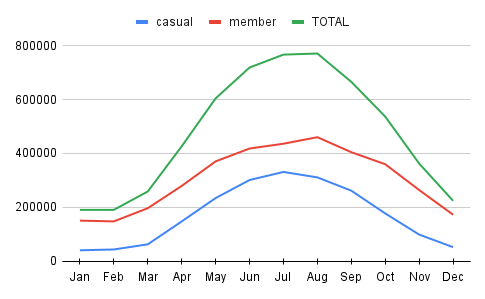
The line chart on the left shows the same but reflects the total counts. Casuals and members both follow similar patterns:
- They become active from February, and this accelerates rapidly from the beginning of March.
- The members reach their peak in August, while the casuals reach theirs in July.
- From those points till December both users are in a downwards trend.
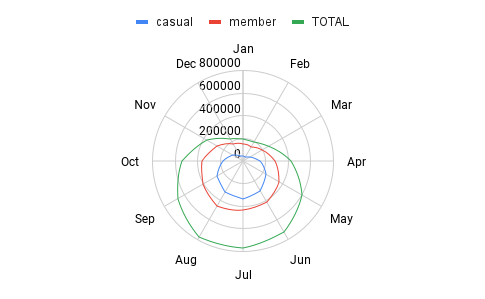
The radar chart on the left has the same information, but with this chart it is clear to see the tendencies as a cycle throughout the year. But for sure this needs to be checked with other years as well. For the year 2023:
- It seems the number of rides are relatively low from beginning of October until the end of March.
- They became more active for the other half of the year, showing a rising up trend from the beginning of April and starting to decrease after August.
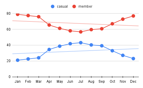
And finally, the line chart on the side shows the proportions within each month separately. Line charts are typically used to show trends over time rather than relative proportions (within a fixed time frame like a month), but here I think this chart is effective to represent the relative trends for different type of users. I normalized the data for each category to percentages (hence proportions) so that the lines represent relative contributions within the month. By this we can tell:
- The members always hold bigger proportions (within any month).
- But the distributions get closer to being equal in the mid of summer.
Things to keep in mind:
- These digits are based on the raw data.
- These are showing the number of rides. The durations of rides may present different insights. I’ll check this on further phase of the EDA.
- These numbers are reflecting the rides, not the distinct users. The number of distinct users may have good amount of impact on the results. Unfortunatelly I can’t dig this deeper, since there is no information about the distinct users, most probably due to privacy issues.
3.2.2 Total Rides by Bike Types in 2023
The below table shows the proportions of the Usage by Bike Types for each month.

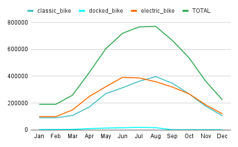
The line chart on the left side shows the same but reflects the total counts.
- Electric Bikes have mostly the biggest counts among all, while the period between July and October being the exception.
- Docked Bikes by the count of ride numbers are relatively quite low.
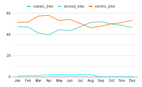
Another way to check this is the line chart on the side, as I did above to show the proportions within each month separately.
- In most months electric bikes seem more popular, except the period mentioned above. This may be caused due to high demand with the sunny days. But just by looking these digits we can not be sure of the reason behind.
Issues with the Docked Bike:
- The term ‘docked bike’ is a bit misleading, because it does not necessarily represent a type of a bike, but a situation of a bike. Any type of bike can be docked. Normally I’d clarify this with the team, but here I can’t and unfortunatelly I couldn’t find any concrete information in their website neither.
- Docked bikes are used only by the Casuals, as we will see below. Therefore, even though I tend to omit them in my further analysis due to their ambiguity, I’ll still keep them into equation simply because they may hold some insights related to the casuals, who are the priority of the business task.
- For the issue mentioned above, I’ll keep my eyes open when it comes to check the durations of the rides.
3.2.3 Total Riders vs Bikes in 2023
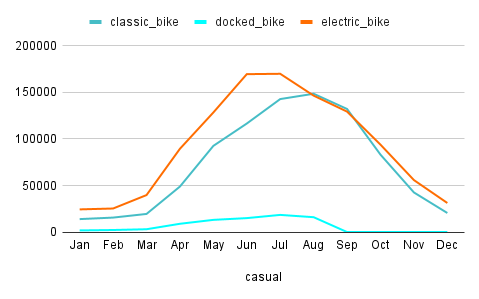
The previous chart shows the total rides
by the Casuals per different bike types.
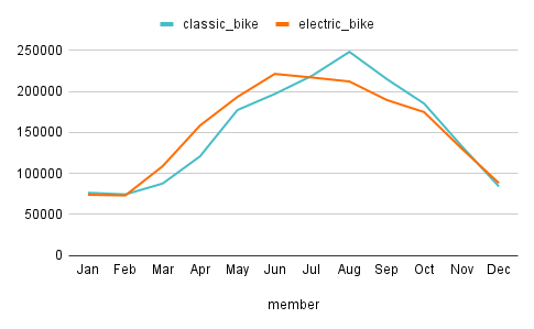
And the next chart shows the total rides
by the Members per different bike types.
- The fact we discovered above that electric-bikes-being-more-popular is much more visible/valid when it comes to the Casuals. Since our business task is mainly focused on the casuals, we have to put this insight into our key takeaway list.
4 Handling the Missing Values & Data Manipulation
Before getting deep into data, let’s first combine all months together and tidy the dataset.
4.1 Combining All CSV Files & Overview
all_trips <- bind_rows(trips_2301, trips_2302, trips_2303, trips_2304,
                       trips_2305, trips_2306, trips_2307, trips_2308,
                       trips_2309, trips_2310, trips_2311, trips_2312)

dim(all_trips)
5719877 13
all_missing_rows <- all_trips %>%
                    filter(!complete.cases(.))
nrow(all_missing_rows)
1388170
There are 5’719’877 observations under 13 variables in total and 1’388’170 of them has minimum one missing value. Their distributions are as follows:
print("Count of all missing values by column")
sapply(all_trips, function(x) sum(is.na(x)))
[1] "Count of all missing values by column"
ride_id0 rideable_type0 started_at0 ended_at0 start_station_name875716 start_station_id875848 end_station_name929202 end_station_id929343 start_lat0 start_lng0 end_lat6990 end_lng6990 member_casual0
Let’s check the consistency once again:
all_trips_station_check <- all_trips %>%
    filter((start_station_name == start_station_name & start_lat != start_lat) |
           (start_station_name == start_station_name & start_lng != start_lng) |
           (end_station_name == end_station_name & end_lat != end_lat) |
           (end_station_name == end_station_name & end_lng != end_lng) |
           (start_station_name == start_station_name & start_station_id != start_station_id) |
           (end_station_name == end_station_name & end_station_id != end_station_id))

nrow(all_trips_station_check)
0
4.2 Handling the Missing Values
Before deciding what to do with the missing values, I want to understand their relationships with each other. Because they all hold information about the stations directly. The skimr library brings good information in that sense, but it requires high CPU. I am not sure I’ll follow the same steps with such a data that holds too much observations.
library(skimr)skim(all_trips) %>%
select(skim_variable, n_missing, complete_rate) %>%
mutate(perct_missing = str_c(round(abs(complete_rate - 1)*100, 2),"%"))A tibble: 13 × 4
| skim_variable | n_missing | complete_rate | perct_missing | |
|---|---|---|---|---|
| <chr> | <int> | <dbl> | <chr> | |
| 1 | started_at | 0 | 1.0000000 | 0% |
| 2 | ended_at | 0 | 1.0000000 | 0% |
| 3 | ride_id | 0 | 1.0000000 | 0% |
| 4 | rideable_type | 0 | 1.0000000 | 0% |
| 5 | start_station_name | 875716 | 0.8468995 | 15.31% |
| 6 | start_station_id | 875848 | 0.8468764 | 15.31% |
| 7 | end_station_name | 929202 | 0.8375486 | 16.25% |
| 8 | end_station_id | 929343 | 0.8375240 | 16.25% |
| 9 | member_casual | 0 | 1.0000000 | 0% |
| 10 | start_lat | 0 | 1.0000000 | 0% |
| 11 | start_lng | 0 | 1.0000000 | 0% |
| 12 | end_lat | 6990 | 0.9987779 | 0.12% |
| 13 | end_lng | 6990 | 0.9987779 | 0.12% |
The missing values regarding to the coordination (lat and lng) can be omitted easily since they are quite low, but around 15% of missing value s not low. Now with the help of naniar library I’ll check how they intersect with each other, as I tried to do in basic EDA phase. I disregarded the missing coordination.
library(naniar)missing_data_upset_table <- all_trips %>%
select(start_station_id, start_station_name, end_station_id, end_station_name)
gg_miss_upset(missing_data_upset_table,
nsets = 4,
nintersects = 10,
main.bar.color = "#43484f",
show.numbers = "yes",
sets.bar.color = "#43484f",
matrix.color = "#a00000",
shade.color = "#97b9f0",
order.by = "freq",
point.size = 3,
line.size = 1,
shade.alpha = 0.2,
text.scale = c(2.5, 1.8, 1.5, 1.3, 1.5, 1.5))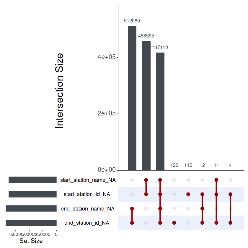
417’110 rows don’t have the information of both start & end stations’ names and ids.
This, of course can be easily (and much more quickly) checked with the code below.
But I wanted to see this visually as I wanted to achieve via Venn diagram in the early phase of my analysis.
missing_stations_demo <- all_trips %>%
    filter(is.na(start_station_name) & is.na(end_station_name))

nrow(missing_stations_demo)
417110
Let’s check how they disperse among the Users and the Bikes:
table(missing_stations_demo$member_casual, missing_stations_demo$rideable_type)classic_bike electric_bike
casual 7 180827
member 21 236255
4.2.1 Side Notes to the Teams: Maintenance and Admin
As the above table reveals, almost all missing-information-about-the-stations come from the electric bike. I’d definitely share this with the teams for future data records to be a complete set without missing values.
4.2.2 What to do with the missing values?
For the following reasons I would not consider to alter the missing values of the stations:
- As I mentioned earlier 15% is too much to avoid or alter without the proper domain knowledge. Normally I’d discuss this with the team and find solutions according to the importance of them.
- Even if we decided to fix the problem and fulfill the missing ones with the true values, there are some issues that may effect our deadlines tremendously. For instance, we could find the missing station names easily if we have the same coordinates matching with some non-missing stations. But then we should ‘widen’ a bit our borders, since these coordinates seem to come from the bike (or maybe even the applications that users are using) not the stations. Even so, there are some odd situations where I checked the coordinates on a map, but found out that they are in the river!
- As below codes reflects, there are 1619 unique station names. Meaning that they are closely located with each other. This leads us again to the importance of the domain knowledge but this time it is not only about the bikes but also about the region, eg. Chicago itself. This is obviously not a single-human job, especially for someone like me who is far away from that city.
- Maybe most importantly: Our business task is clearly focused on converting the casuals into members. Therefore it would make much more sense to focus users’ behaviour first. (Maybe later on widen those insights from the initial analysis to the regions to come up much more comprehensive work.)
Having said that, while I won’t focus on the stations further on, I’ll still keep them (only the names of them) in the dataset just to have at least a broader sense of their popularity (hence to understand which stations are more active).
unique_start_station <- all_trips %>%
    select(start_station_name) %>%
    unique() %>%
    pull()

unique_end_station <- all_trips %>%
    select(end_station_name) %>%
    unique() %>%
    pull()

unique_stations <- c(unique_start_station, unique_end_station) %>%
  unique()

length(unique_stations)
1619
4.3 Data Manipulation: Checking the Durations of the Bike Trips
Let’s add a column to check the durations of the rides. But first, are all the end-times come after the start-times?
trips_dur <- all_trips %>%
    mutate(duration_sec = as.numeric(ended_at - started_at)) %>%
    arrange(duration_sec)

head(trips_dur)| ride_id | rideable_type | started_at | ended_at | start_station_name | start_station_id | end_station_name | end_station_id | start_lat | start_lng | end_lat | end_lng | member_casual | duration_sec |
|---|---|---|---|---|---|---|---|---|---|---|---|---|---|
| <chr> | <chr> | <dttm> | <dttm> | <chr> | <chr> | <chr> | <chr> | <dbl> | <dbl> | <dbl> | <dbl> | <chr> | <dbl> |
| F584D47AE67FD388 | classic_bike | 2023-11-05 21:08:17 | 2023-10-25 07:31:46 | Sheffield Ave & Waveland Ave | TA1307000126 | NA | NA | 41.94929 | -87.65446 | 41.95 | -87.65 | casual | -999391 |
| AE046C379C20B7CA | classic_bike | 2023-11-05 20:46:59 | 2023-10-25 07:31:46 | Sheridan Rd & Irving Park Rd | 13063 | NA | NA | 41.95430 | -87.65440 | 41.95 | -87.65 | member | -998113 |
| A21D6507DA3C5AD4 | classic_bike | 2023-11-05 16:41:54 | 2023-10-25 07:31:46 | Pine Grove Ave & Irving Park Rd | TA1308000022 | NA | NA | 41.95440 | -87.64805 | 41.95 | -87.65 | member | -983408 |
| DEC5EF8DE27398A0 | classic_bike | 2023-11-05 11:56:19 | 2023-10-25 07:31:46 | Pine Grove Ave & Irving Park Rd | TA1308000022 | NA | NA | 41.95436 | -87.64811 | 41.95 | -87.65 | casual | -966273 |
| 7850F6E2343BF766 | classic_bike | 2023-11-01 16:38:10 | 2023-10-25 07:31:46 | Clark St & Drummond Pl | TA1307000142 | NA | NA | 41.93119 | -87.64421 | 41.93 | -87.64 | casual | -637584 |
| 5A5DDAFFF234FB69 | classic_bike | 2023-11-01 14:07:31 | 2023-10-25 07:31:46 | Clark St & Drummond Pl | TA1307000142 | NA | NA | 41.93118 | -87.64417 | 41.93 | -87.64 | member | -628545 |
There are minus durations indeed! Let’s investigate deeper. I’ll start with the negative and minimum values.
# Total observations with negative durations
trips_dur_neg <- trips_dur %>%
    filter(duration_sec < 0)

nrow(trips_dur_neg)
272
Normally I would discuss this with the team but now since 272 observations compared to over 5 million ones is quite low I won’t assume anything, (hence I won’t try to convert end and start times into each other) and eliminate those rows instead.
Now let’s check those durations that are quite short for a bike ride, because there are some durations that are only for a second! Again normally I’d communicate with the team but here I’ll assume that durations shorter than a minute are not realistic, by adopting the ideas like “riders trying to figure out how to dock-undock bikes” or some issues that might come up with the application.*
*On their website they have instructions to show how to dock a bike (here is the link), and they use terms like “insert your bike gently but firmly” or “holding the bike in place for at least 5 seconds”, meaning having an issue while docking may be not an uncommon thing indeed!
But anyway I’ll investigate this section (durations that are 0-60 secs) in two sub-sections for the sake of a deeper research.
# Total observations with durations equal or shorter than half a minute that are not negative
trips_dur_0s30s <- trips_dur %>%
    filter(duration_sec >= 0 & duration_sec < 31)

nrow(trips_dur_0s30s)
str_c(round(nrow(trips_dur_0s30s)/nrow(trips_dur)*100, 2),"%")
97726
'1.71%'
The first part (durations that are 0-30 sec) hold less than 2% of the whole observations.
# Total observations with durations 31-59 sec
trips_dur_31s59s <- trips_dur %>%
    filter(duration_sec > 30 & duration_sec < 60)

nrow(trips_dur_31s59s)
str_c(round(nrow(trips_dur_31s59s)/nrow(trips_dur)*100, 2),"%")
51617
'0.9%'
The second part (durations that are 31-59 sec) hold less than 1% of the whole observations. Let’s check how many of them have the same end and start station names, assuming that they are coming from the users who had similar issues described above.
trips_dur_31s59s_stat <- trips_dur_31s59s %>%
    filter((start_station_name == end_station_name) |
           (start_station_id == end_station_id))

nrow(trips_dur_31s59s_stat)
str_c(round(nrow(trips_dur_31s59s_stat)/nrow(trips_dur_31s59s)*100, 2),"%")
28412
'55.04%'
More than half of them occurred in the same station. But let’s be sure that all the rest are started from one station but ended in another one or not.
trips_dur_31s59s_stat_not <- trips_dur_31s59s %>%
    filter((start_station_name != end_station_name) |
           (start_station_id != end_station_id))

nrow(trips_dur_31s59s_stat_not)
str_c(round(nrow(trips_dur_31s59s_stat_not)/nrow(trips_dur_31s59s)*100, 2),"%")
3138
'6.08%'
In fact, it looks like that it’s not always the case or we can’t be sure, because the remaining of this section (that are ~40%) comes with NAs. I guess at this point it is safe to omit all records that are under a minute. But again, normally I’d talk this over with the team.
Now let’s check the tail to observe maximum values.
# Total observations with durations longer than a day
trips_dur_day <- trips_dur %>%
    filter(duration_sec > 60*60*24)

nrow(trips_dur_day)
str_c(round(nrow(trips_dur_day)/nrow(trips_dur)*100, 2),"%")
6418
'0.11%'
Total observations with durations longer than a day are very low with only 6418 rows. That’s not much compared to whole number of observations, but out of curiousity I’ll check trips that are longer than a week and a month, if they exist.
# Total observations with durations longer than a week
trips_dur_week <- trips_dur %>%
    filter(duration_sec > 60*60*24*7)

nrow(trips_dur_week)
363
# Total observations with durations longer than a month
trips_dur_mon <- trips_dur %>%
    filter(duration_sec > 60*60*24*30)

nrow(trips_dur_mon)
11
Even it is too rare (hence outliers), we DO have durations of trips that are longer than a month! Let’s check by whom and with what type of bikes they are.
# Distribution of users and bikes that have a trip-duration longer than a day
table(trips_dur_day$member_casual, trips_dur_day$rideable_type)
classic_bike docked_bike
casual 3803 1460
member 1155 0
Durations longer than a day are done by casuals more than members, even though they are without a subscription. Although there are not many longer-than-a-day-casuals, still this may be used as a marketing strategy.
“Hey, what a ride! This is the second time you ride longer than a day. Well done!
Would you like to consider a membership to benefit from this even more?“
4.4 Eliminating values and dropping out variables
I’ll shorten the data by dropping out the columns about stations except the names of the start and end stations.
trips_short <- trips_dur %>%
    select(member_casual, rideable_type, duration_sec, started_at, ended_at, start_station_name, end_station_name)

head(trips_short)| member_casual | rideable_type | duration_sec | started_at | ended_at | start_station_name | end_station_name |
|---|---|---|---|---|---|---|
| <chr> | <chr> | <dbl> | <dttm> | <dttm> | <chr> | <chr> |
| casual | classic_bike | -999391 | 2023-11-05 21:08:17 | 2023-10-25 07:31:46 | Sheffield Ave & Waveland Ave | NA |
| member | classic_bike | -998113 | 2023-11-05 20:46:59 | 2023-10-25 07:31:46 | Sheridan Rd & Irving Park Rd | NA |
| member | classic_bike | -983408 | 2023-11-05 16:41:54 | 2023-10-25 07:31:46 | Pine Grove Ave & Irving Park Rd | NA |
| casual | classic_bike | -966273 | 2023-11-05 11:56:19 | 2023-10-25 07:31:46 | Pine Grove Ave & Irving Park Rd | NA |
| casual | classic_bike | -637584 | 2023-11-01 16:38:10 | 2023-10-25 07:31:46 | Clark St & Drummond Pl | NA |
| member | classic_bike | -628545 | 2023-11-01 14:07:31 | 2023-10-25 07:31:46 | Clark St & Drummond Pl | NA |
Now I’ll remove the observations that are shorter than a minute, as I described above on the initial EDA.
trips_short_drop <- subset(trips_short, duration_sec >= 60)
nrow(trips_short_drop)
5570262
# Checking the new distribution
table(trips_short_drop$member_casual, trips_short_drop$rideable_type)
classic_bike docked_bike electric_bike
casual 864555 77574 1063621
member 1790185 0 1774327
count_docked <- nrow(trips_short_drop[trips_short_drop$rideable_type == "docked_bike",])
count_bikes <- nrow(trips_short_drop[!is.na(trips_short_drop$rideable_type),])

str_c(round(count_docked / count_bikes *100,2),"%")
'1.39%'
Docked Bikes hold a little higher than 1% of total number of rides. In a normal scenario, I’d discuss this with the team, but since there are no records regarding the docked bikes after September and their percentage is relatively low I’d tend to omit them. But first, let’s check how they contribute to the total duration:
bike_durations <- trips_short_drop %>%
    group_by(rideable_type) %>%
    summarise(total_dur_month=sum(duration_sec/60/60/24/30),
             .groups = 'drop')

head(bike_durations)| rideable_type | total_dur_month |
|---|---|
| <chr> | <dbl> |
| classic_bike | 1237.0742 |
| docked_bike | 331.2884 |
| electric_bike | 838.0037 |
That’s suprizing! Even though they hold quite less amount of rides, their durations are holding much bigger proportion. Their durations are roughly 40% compared to the Electric Bikes’ and roughly one quarter of the Classic Bikes’ total durations. They are a little less than 14% of the total durations.
As I explained before, since it is not clear for me what does ‘docked bike’ really mean (another type of bike or one of electric-or-classic that are not docked to a station), I’d still omit them but I will keep them into the equations to have a better sense of what is going on with them. Because only casuals are using them and this may give me some insights.
summary(trips_short_drop$duration_sec/60)Min. 1st Qu. Median Mean 3rd Qu. Max.
1.00 5.70 9.80 18.66 17.23 98489.07
According to the digits above, (for the durations of the trips) it looks like median (that is slightly less than 10 min) is a better measure here of central tendency, rather than the mean.
5 Further EDA
5.1 Checking the Stations
Before I leave the stations totally behind the analysis, I’d quickly check the busiest start and end stations anyway. This may give some directions for future researches. I won’t do anything about the missing values though.
top_10_start_station <- trips_short_drop %>%
  mutate(start_station_name = fct_lump(start_station_name, 10)) %>%
  count(start_station_name, name = "counts", sort = T) %>%
  filter(!is.na(start_station_name),
         start_station_name != "Other") %>%
  mutate(start_station_name = fct_reorder(start_station_name, counts))

top_10_start_station| start_station_name | counts |
|---|---|
| <fct> | <int> |
| Streeter Dr & Grand Ave | 61952 |
| DuSable Lake Shore Dr & Monroe St | 39462 |
| Michigan Ave & Oak St | 36583 |
| Clark St & Elm St | 35138 |
| DuSable Lake Shore Dr & North Blvd | 35133 |
| Kingsbury St & Kinzie St | 34288 |
| Wells St & Concord Ln | 32960 |
| Clinton St & Washington Blvd | 31991 |
| Wells St & Elm St | 29917 |
| Millennium Park | 29488 |
# installing packages to be able to use unit_format
install.packages("scales")
library(scales)
top_10_start_station_plt <- ggplot(head(top_10_start_station, 10)) +
geom_col(aes(start_station_name, counts, fill = start_station_name),
width = 0.8,
show.legend = FALSE) +
coord_flip() +
#scale_x_continuous(position = "top") +
scale_y_continuous(labels = unit_format(unit = "K", scale = 1e-3), trans = "reverse") +
scale_fill_viridis_d(option = "mako", direction = -1) +
labs(title = "Most Visited Start Stations",
x = NULL,
y = NULL) +
theme_gray(base_size = 14)
top_10_start_station_plt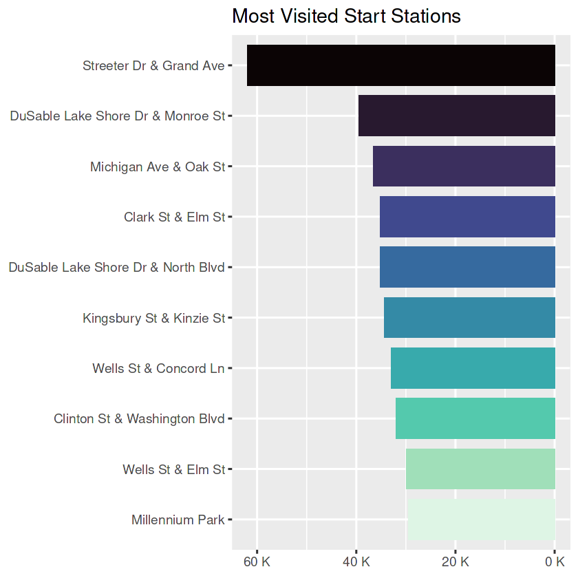
top_10_end_station <- trips_short_drop %>%
  mutate(end_station_name = fct_lump(end_station_name, 10)) %>%
  count(end_station_name, name = "counts", sort = T) %>%
  filter(!is.na(end_station_name),
         end_station_name != "Other") %>%
  mutate(end_station_name = fct_reorder(end_station_name, counts))

top_10_end_station| end_station_name | counts |
|---|---|
| <fct> | <int> |
| Streeter Dr & Grand Ave | 63061 |
| DuSable Lake Shore Dr & North Blvd | 38695 |
| Michigan Ave & Oak St | 37291 |
| DuSable Lake Shore Dr & Monroe St | 37253 |
| Clark St & Elm St | 34369 |
| Kingsbury St & Kinzie St | 33692 |
| Wells St & Concord Ln | 33620 |
| Clinton St & Washington Blvd | 32698 |
| Millennium Park | 30436 |
| Theater on the Lake | 30094 |
top_10_end_station_plt <- ggplot(head(top_10_end_station, 10)) +
  geom_col(aes(end_station_name, counts, fill = end_station_name),
           width = 0.8,
           show.legend = FALSE) +
  coord_flip() +
  scale_y_continuous(labels = unit_format(unit = "K", scale = 1e-3)) +
  scale_fill_viridis_d(option = "mako", direction = -1) +
  labs(title = "Most Visited End Stations",
       x = NULL,
       y = NULL) +
  theme_gray(base_size = 14)

top_10_end_station_plt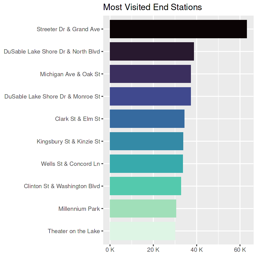
Now let’s repeat the same process for the durations.
longest_dur_stations_start <- trips_short_drop %>%
    group_by(start_station_name) %>%
    summarise(Freq = sum(duration_sec)) %>%
    filter(!is.na(start_station_name)) %>%
    arrange(-Freq) %>%
    mutate(start_station_name = fct_reorder(start_station_name, Freq))

longest_dur_stations_start_plt <- ggplot(head(longest_dur_stations_start, 10)) +
  geom_col(aes(start_station_name, Freq, fill = start_station_name),
           width = 0.8,
           show.legend = FALSE) +
  coord_flip() +
  scale_y_continuous(labels = unit_format(unit = "K", scale = 1e-3)) +
  scale_fill_viridis_d(option = "mako", direction = -1) +
  labs(title = "Start Stats with Longest Ride Durations",
       x = NULL,
       y = NULL) +
  theme_gray(base_size = 14)

longest_dur_stations_start_plt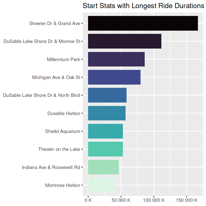
longest_dur_stations_end <- trips_short_drop %>%
    group_by(end_station_name) %>%
    summarise(Freq = sum(duration_sec)) %>%
    filter(!is.na(end_station_name)) %>%
    arrange(-Freq) %>%
    mutate(end_station_name = fct_reorder(end_station_name, Freq))

longest_dur_stations_end_plt <- ggplot(head(longest_dur_stations_end, 10)) +
  geom_col(aes(end_station_name, Freq, fill = end_station_name),
           width = 0.8,
           show.legend = FALSE) +
  coord_flip() +
  scale_y_continuous(labels = unit_format(unit = "K", scale = 1e-3)) +
  scale_fill_viridis_d(option = "mako", direction = -1) +
  labs(title = "End Stats with Longest Ride Durations",
       x = NULL,
       y = NULL) +
  theme_gray(base_size = 14)

longest_dur_stations_end_plt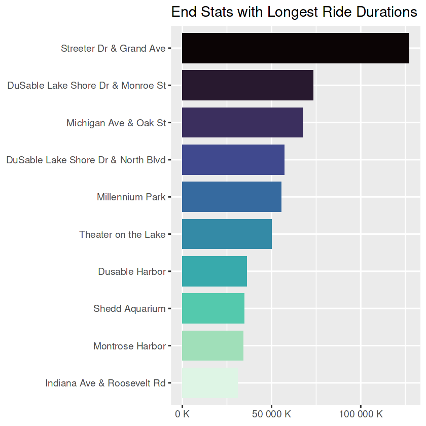
5.1.1 Combining the Plots
To get different insights I combined the above plots in two groups. First, I matched the start and end stations and second, I matched the counts and the durations.
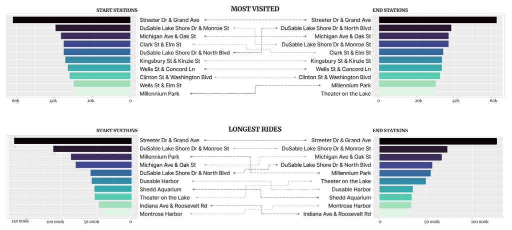
- By far, ‘Streeter Dr & Grand Ave’ is the most visited station and also holds the longest rides. If Marketing Team aims big mass, this station could be the starting point for ads.
- Top 10 of start and end stations in both scenarios (most visited or the longest trips) are the same stations, with two exceptions (in most visited list: Wells St & Elm St and Theater on the Lake) and with some minor ranking differences.
- These top 10 lists could be a good starting point if the Marketing Team plans to have actions in the stations. OR with the future analysis, other stations that are not listed here could be analyzed.
Now let’s check the start and end stations separately.
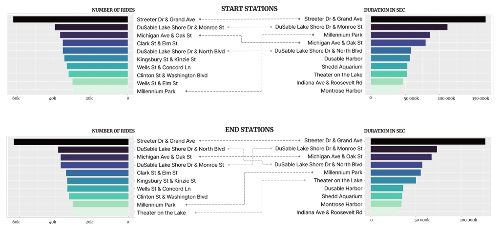
- For both start and end stations, the most visited ones do not necessarily hold the longest trips.
- Those stations that holds longer trips compared to the number of rides could be used for targeted ads. The same could be implied for those that have much visits but hold relatively shorter trips.
From this moment on, I followed two parallel paths:
- Saved the recent file as csv and loaded to Tableau to get my charts there.
- Continued with R to plot the charts in Jupyter.
write.csv(trips_short_drop, "trips_short.csv", row.names = F)5.2 EDA on Bike Trips (Total Number of Rides and their Durations)
Further I’ll examine the total numbers of rides and their durations.
5.2.1 Bike Trips per Month
month_count <- trips_short_drop %>%
   group_by(month=floor_date(started_at, "month")) %>%
   summarize(n())

month_count| month | n() |
|---|---|
| <dttm> | <int> |
| 2023-01-01 | 184113 |
| 2023-02-01 | 184444 |
| 2023-03-01 | 249601 |
| 2023-04-01 | 411607 |
| 2023-05-01 | 586955 |
| 2023-06-01 | 700835 |
| 2023-07-01 | 747487 |
| 2023-08-01 | 753322 |
| 2023-09-01 | 652054 |
| 2023-10-01 | 525420 |
| 2023-11-01 | 355114 |
| 2023-12-01 | 219310 |
month_duration <- trips_short_drop %>%
   group_by(month=floor_date(started_at, "month")) %>%
   summarize(amount_min=sum(duration_sec/60))

month_duration| month | amount_min |
|---|---|
| <dttm> | <dbl> |
| 2023-01-01 | 2471706 |
| 2023-02-01 | 2575004 |
| 2023-03-01 | 3380157 |
| 2023-04-01 | 7336136 |
| 2023-05-01 | 11504845 |
| 2023-06-01 | 14373298 |
| 2023-07-01 | 16678734 |
| 2023-08-01 | 17300426 |
| 2023-09-01 | 11903288 |
| 2023-10-01 | 8419332 |
| 2023-11-01 | 5010795 |
| 2023-12-01 | 3001302 |
Plotting the Bike Trips per Month
month_count <- trips_short_drop %>%
  select(member_casual, started_at) %>%
  drop_na(started_at, member_casual) %>%
  mutate(month = month(started_at)) %>%
  group_by(month, member_casual) %>%
  summarise(counts = n(),
            .groups = "drop") %>%
  ungroup() %>%
  ggplot() +
  geom_line(aes(month, counts, color = member_casual),
            size = 2) +
  scale_x_continuous(breaks = c(1,2,3,4,5,6,7,8,9,10,11,12),
    labels = c("Jan", "Feb", "Mar", "Apr", "May", "Jun", "Jul", "Aug", "Sep", "Oct", "Nov", "Dec")) +
  scale_y_continuous(labels = unit_format(unit = "K", scale = 1e-3)) +
  scale_color_manual(
    name = NULL,
    values = c("casual" = "#4285f4", "member" = "#ea4335"),
    labels = c("Casual", "Member")
  ) +
  theme(legend.position = "bottom") +
  labs(title = "Total no. of Rides by Month per Users",
       x = NULL,
       y = NULL)

month_count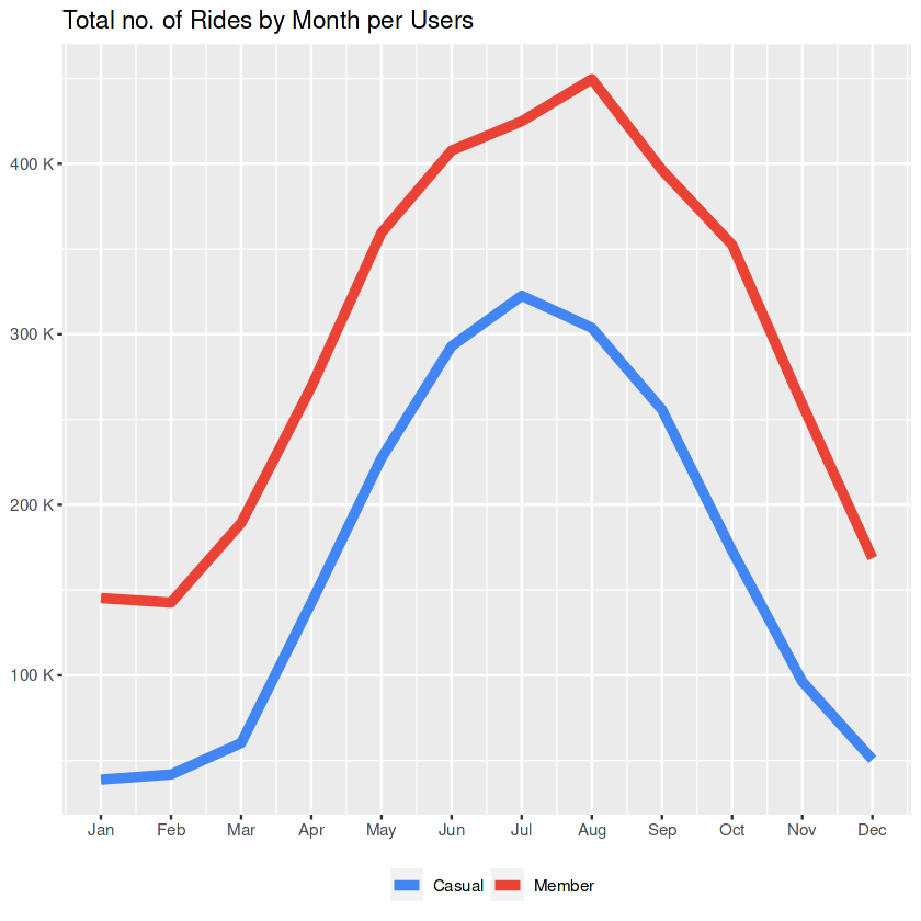
This graph is pretty close to the one that we created earlier with the raw data. Casuals and members both follow similar patterns:
- They become active starting from February, and this accelerates rapidly from the beginning of March.
- The members reach their peak in August, while the casuals reach theirs in July.
- From those points till December both users are in a downwards trend.
Side Notes to the Marketing Team:
- Being active before sunny seasons may help to convert casuals into members.
- Offerings during the autumn may help to keep the customers more active.
Now, let’s check the situation with the durations.
month_duration <- trips_short_drop %>%
  select(member_casual, started_at, duration_sec) %>%
  drop_na(started_at, member_casual) %>%
  mutate(month = month(started_at)) %>%
  group_by(month, member_casual) %>%
  summarise(amount_min=sum(duration_sec/60)) %>%
  ungroup() %>%
  arrange(desc(amount_min)) %>%
  ggplot() +
  geom_line(aes(month, amount_min, color = member_casual),
            size = 2) +
  scale_x_continuous(breaks = c(1,2,3,4,5,6,7,8,9,10,11,12),
    labels = c("Jan", "Feb", "Mar", "Apr", "May", "Jun", "Jul", "Aug", "Sep", "Oct", "Nov", "Dec")) +
  scale_y_continuous(labels = unit_format(unit = "K", scale = 1e-3)) +
  scale_color_manual(
    name = NULL,
    values = c("casual" = "#4285f4", "member" = "#ea4335"),
    labels = c("Casual", "Member")
  ) +
  theme(legend.position = "bottom") +
  labs(title = "Total Duration of the Rides by Month per Users",
       x = NULL,
       y = NULL)

month_duration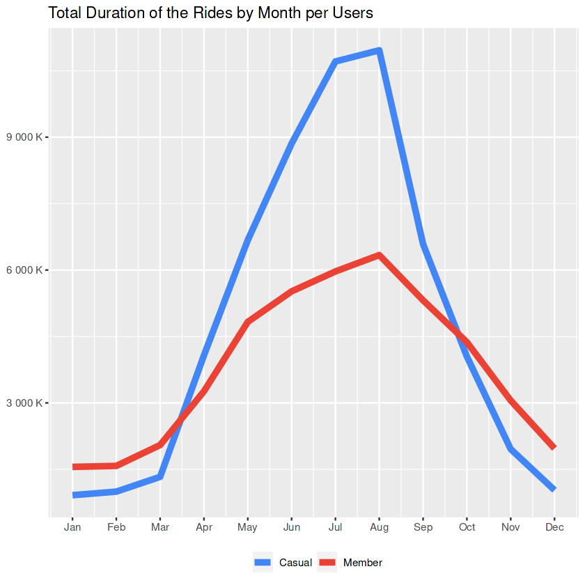
That’s interesting!
Even the number of rides by casuals were always less than the numbers of rides by the members, the period from April to October has trips with much longer durations, that are done by casuals.
Side Notes to the Marketing Team:
- Membership offers, that specialized to the casuals who are doing long trips may help to convince them to subscribe.
- Above notes about sunny seasons are still valid.
But let’s also check the effect of the ‘docked bikes’ in this regard.
month_duration_no_dock <- trips_short_drop %>%
  select(member_casual, started_at, duration_sec, rideable_type) %>%
  drop_na(started_at, member_casual) %>%
  filter(rideable_type == "classic_bike" | rideable_type == "electric_bike") %>%
  mutate(month = month(started_at)) %>%
  group_by(month, member_casual) %>%
  summarise(amount_min=sum(duration_sec/60)) %>%
  ungroup() %>%
  arrange(desc(amount_min)) %>%
  ggplot() +
  geom_line(aes(month, amount_min, color = member_casual),
            size = 2) +
  scale_x_continuous(breaks = c(1,2,3,4,5,6,7,8,9,10,11,12),
    labels = c("Jan", "Feb", "Mar", "Apr", "May", "Jun", "Jul", "Aug", "Sep", "Oct", "Nov", "Dec")) +
  scale_y_continuous(labels = unit_format(unit = "K", scale = 1e-3)) +
  scale_color_manual(
    name = NULL,
    values = c("casual" = "#4285f4", "member" = "#ea4335"),
    labels = c("Casual", "Member")
  ) +
  theme(legend.position = "bottom") +
  labs(title = "Total Duration of the Rides (excl. docked bike) by Month per Users",
       x = NULL,
       y = NULL)

month_duration_no_dock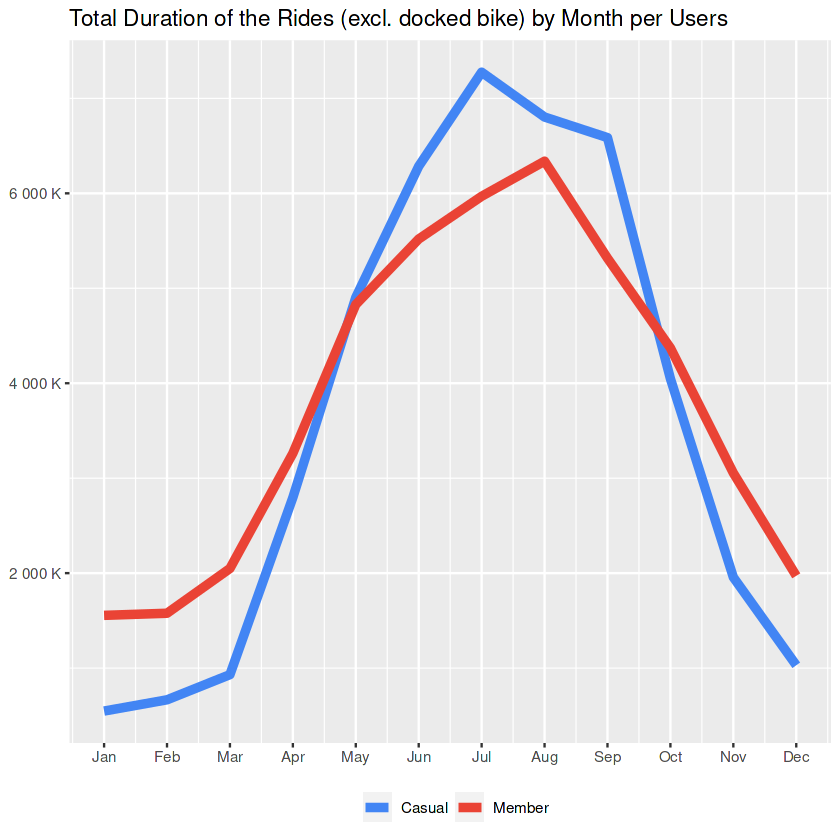
The situation with the previous chart (that casuals holding longer trips during sunny seasons) is less strong if we take the docked bike out of the equation.
So whatever-the-docked-bikes-are-offering may contribute to having longer trips by casuals.
Side Notes to the Marketing Team:
- A further study on docked bikes may reveal some insights about the usage and this may help to create some opportunities.
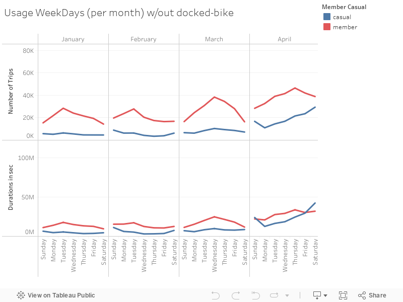
5.2.2 Bike Trips per Weekdays
Let’s check the distribution during weekdays as well.
day_count <- trips_short_drop %>%
  select(member_casual, started_at) %>%
  drop_na(started_at, member_casual) %>%
  mutate(weekday = wday(started_at)) %>%
  group_by(weekday, member_casual) %>%
  summarise(counts = n(),
            .groups = "drop") %>%
  ungroup() %>%
  arrange(desc(counts)) %>%
  ggplot() +
  geom_path(aes(weekday, counts, color = member_casual),
            size = 2) +
  scale_x_continuous(breaks = c(1,2,3,4,5,6,7),
    labels = c("Sun", "Mon", "Tue", "Wed", "Thu", "Fri", "Sat")) +
  scale_y_continuous(labels = unit_format(unit = "K", scale = 1e-3)) +
  scale_color_manual(
    name = NULL,
    values = c("casual" = "#4285f4", "member" = "#ea4335"),
    labels = c("Casual", "Member")
  ) +
  theme(legend.position = "bottom") +
  labs(title = "Total no. of the Rides by Weekdays per Users",
       x = NULL,
       y = NULL)

day_count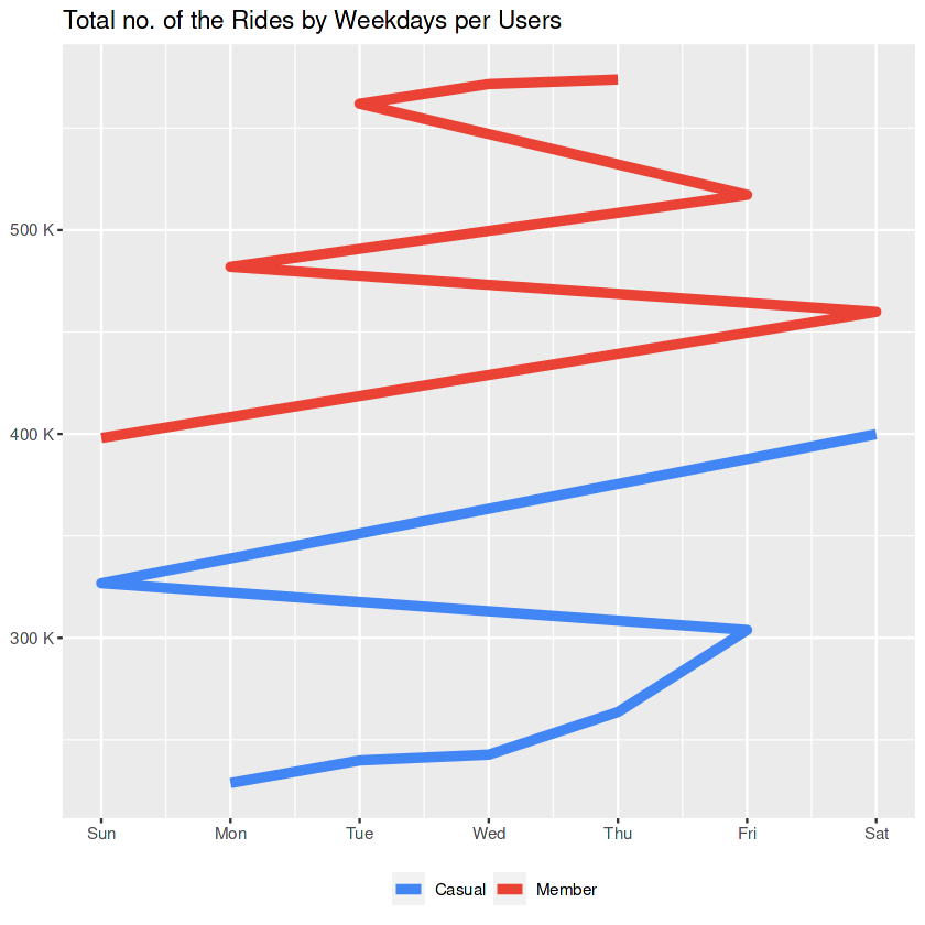
The geom_path clearly shows the hieararchy when it comes to revealing the busiest days.
- Members are more active on weekdays, casuals are more active on weekends.
- Members using the service mostly on workdays, hence they might relate it to their jobs.
- Members are most active on Thursday, Wednesday and Tuesday; casuals are most active on Saturday and Sunday.
- Following their most active days both groups are most active on Fridays.
Side Notes to the Marketing Team:
- Since members are more active on weekdays, new offerings to casuals related to their jobs can be considered.
- Fridays have potentials for both group. Targeted ads for members can underline “the end of the week”, ads for casuals can underline “the beginning of the weekend”.
Let’s check the durations as well.
day_duration <- trips_short_drop %>%
  select(member_casual, started_at, duration_sec) %>%
  drop_na(started_at, member_casual) %>%
  mutate(weekday = wday(started_at)) %>%
  group_by(weekday, member_casual) %>%
  summarise(amount_min=sum(duration_sec/60)) %>%
  ungroup() %>%
  arrange(desc(amount_min)) %>%
  ggplot() +
  geom_line(aes(weekday, amount_min, color = member_casual),
            size = 2) +
  scale_x_continuous(breaks = c(1,2,3,4,5,6,7),
    labels = c("Sun", "Mon", "Tue", "Wed", "Thu", "Fri", "Sat")) +
  scale_y_continuous(labels = unit_format(unit = "K", scale = 1e-3)) +
  scale_color_manual(
    name = NULL,
    values = c("casual" = "#4285f4", "member" = "#ea4335"),
    labels = c("Casual", "Member")
  ) +
  theme(legend.position = "bottom") +
  labs(title = "Total Duration of the Rides by Weekdays per Users",
       x = NULL,
       y = NULL)

day_duration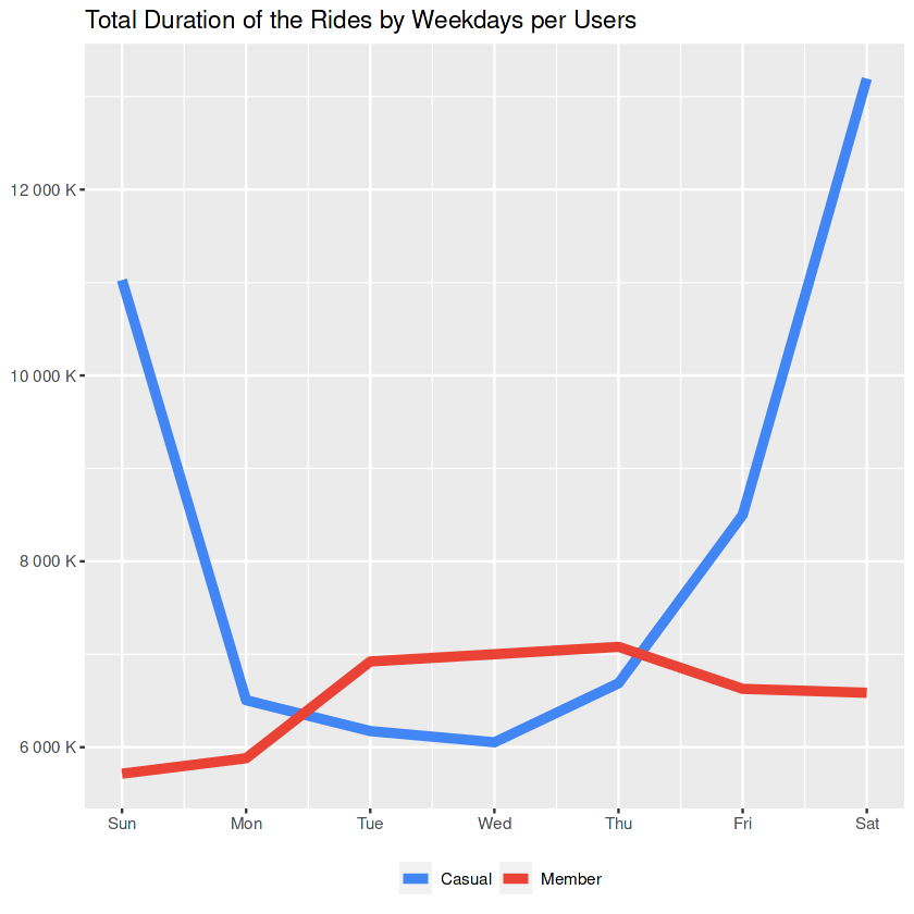
This line chart shows that the casuals are using the service for longer trips on weekends.
Side Notes to the Marketing Team:
- New type of membership that focuses on weekend-usage can be introduced.
- Above notes about Friday and weekdays are still valid.
“Yes we don’t like the workdays either, but you don’t have to say goodbye to our bikes on weekdays!“
Checking Days: Deeper Investigation for Future Studies
With Tableau it is relatively easier to create complicated charts like the one below. With this chart the daily distributions within each month can be studied for further analysis.
- Notice the durations by Casuals in September, compared to other months. That could be a new insight. (But to keep this study simpler, for now I won’t dig deeper any further. This is another side note to the Marketing Team.)
5.2.3 Bike Trips Throughout a Day
And lastly, let’s check the daily distributions, focusing on each hour.
hours_count <- trips_short_drop %>%
  select(member_casual, started_at) %>%
  drop_na(started_at, member_casual) %>%
  mutate(hour = hour(started_at)) %>%
  group_by(hour, member_casual) %>%
  summarise(counts = n(),
            .groups = "drop") %>%
  ungroup() %>%
  arrange(desc(counts)) %>%
  ggplot() +
  geom_line(aes(hour, counts, color = member_casual),
            size = 2) +
  scale_x_continuous(breaks = c(0,1,2,3,4,5,6,7,8,9,10,11,12,13,14,15,16,17,18,19,20,21,22,23),
                     labels = c("00","01","02","03","04","05","06","07","08","09","10","11","12","13","14","15","16","17","18","19","20","21","22","23")) +
  scale_y_continuous(labels = unit_format(unit = "K", scale = 1e-3)) +
  scale_color_manual(
    name = NULL,
    values = c("casual" = "#4285f4", "member" = "#ea4335"),
    labels = c("Casual", "Member")
  ) +
  theme(legend.position = "bottom") +
  labs(title = "Total no. of the Rides during the day per Users",
       x = NULL,
       y = NULL)

hours_count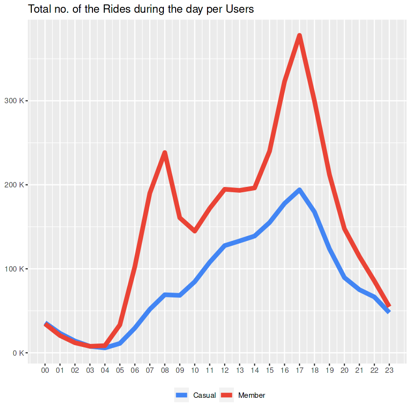
This graph supports our previous assumption about “the members that they use the service mostly because of their job”. They are most active when the working hours start and end.
Side Notes to the Marketing Team:
- It seems that the end of a working day has a potential for both groups.
- Since both group’s peak point is same at 17:00, we might say that casuals’ usages could be related to their jobs too.
Let’s check the duration throughout the day as well.
hours_duration <- trips_short_drop %>%
  select(member_casual, started_at, duration_sec) %>%
  drop_na(started_at, member_casual) %>%
  mutate(hour = hour(started_at)) %>%
  group_by(hour, member_casual) %>%
  summarise(amount_min=sum(duration_sec/60)) %>%
  ungroup() %>%
  arrange(desc(amount_min)) %>%
  ggplot() +
  geom_line(aes(hour, amount_min, color = member_casual),
            size = 2) +
  scale_x_continuous(breaks = c(0,1,2,3,4,5,6,7,8,9,10,11,12,13,14,15,16,17,18,19,20,21,22,23),
                     labels = c("00","01","02","03","04","05","06","07","08","09","10","11","12","13","14","15","16","17","18","19","20","21","22","23")) +
  scale_y_continuous(labels = unit_format(unit = "K", scale = 1e-3)) +
  scale_color_manual(
    name = NULL,
    values = c("casual" = "#4285f4", "member" = "#ea4335"),
    labels = c("Casual", "Member")
  ) +
  theme(legend.position = "bottom") +
  labs(title = "Total Duration of the Rides during the day per Users",
       x = NULL,
       y = NULL)

hours_duration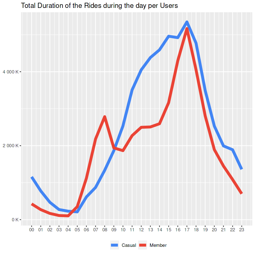
It is clear that the period between 17:00-18:00 is the most busiest one with the longest trip durations in a day.
Side Notes to the Marketing Team:
- Focusing on ‘ending a work day’ in an ad campaign might help to gain more members.
“End of a tough day? You deserve to ride a bike!“
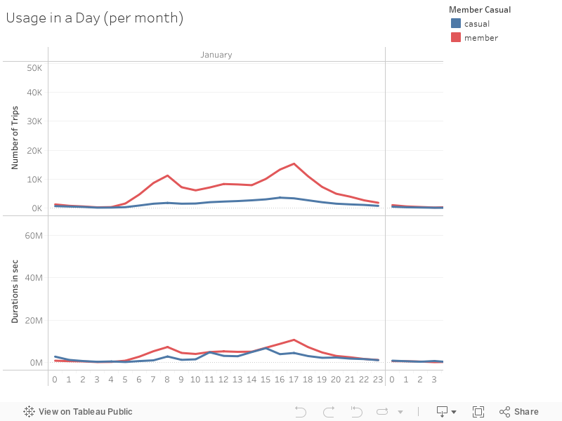
Checking Hours: Deeper Investigation for Future Studies
Again we can use Tableau charts for a deeper investigation. With the below chart the hourly distributions within each month can be studied for further analysis.
- Notice how the Members’ pattern keep being consistent throughout the year, for both the number of trips and their durations.
6 Conclusion
6.1 Let’s summarize the key takeaways
- Both members and casuals are most active during summer, followed by spring and autumn.
- Casuals tend to have longer trips, especially during summer.
- Docked-bikes have a great effect on longer trips by casuals.
- While weekdays members are more active, on weekends casuals are more active.
- Following the above, second busiest period of the week for both group is Friday.
- During the day most active time for both group is between 17:00 and 18:00.
6.2 Solutions for Marketing Team
Based on the insights above the below scenarios can be considered for advertising campaign.
Scenario 1: Seasonal, wider-focus on all users
- Come up with offerings that are focusing on summer usages. For this the period Jan-Feb may be better than Oct-Dec, because the first one has a neutral tendency, compared to the downward trend on the latter one.
- There might be another focus on autumn to postpone the ‘summer effect’ on the usages.
Scenario 2: Seasonal, narrow-focus on casuals
- New kind of membership for those who like to have longer trips can be offered.
- Main motivation for this could be summer usages.
Scenario 3: Case-based, narrow-focus on bike types (requires further analyses)
- Study the docked bikes for future possiblities, since they hold good amount of longer trips by casuals.
- For this, we will need to have the data about the type of bikes and the users.
Scenario 4: Theme-based, narrow-focus on casuals
- Since members clearly follows working hours/days pattern and casuals too show some similar signs, targetting marketing focusing on working rituals can be used.
- For this, Fridays could be used as a good accelarator point.
Scenario 5: Periodic, narrow-focus on casuals
- Similar to Scenario 2, memberships could be introduced to underline the usage on weekends and/or the end of a working day.
- Main motivation for this could be longer trips that casuals tend to have.
7 Next Steps
Considering that the main focus of the business task is being to convert casuals into members, from above Scenario 2 and Scenario 5 or a combination of both can be used. Because both scenario’s main focuses are casuals and they don’t require additional studies, although it would be wise to continue with the analysis via upcoming data inputs parallelly.
A wider, seasonal ‘summer campaign’ can be combined with a periodic one, that feeds itself with the working rituals. This way, a consistent wider concept might work together with a more dynamic one, that follows promising trends. While the first one could rely on static places, like stations or directly bikes; the latter one could benefit from the mobile devices.
Previous Data Project

Next Data Project

Browse my projects by category:
ALL • Data • UX • Arch