
My role
Data Analysis & Research
Performing a detailed EDA, building ML Models

Timeline
Jan ’25
Final Assignment, BSBI
MSc Data Analytics

Tools
Python
Jupyter
Office Suite
OVERVIEW
The Data
The Bitcoin Dataset holds different attributes for daily price changes.
The Goal
I’ll model three different regression algorithms to predict the Bitcoin prices.
Tools
Pandas and Numpy for basics,
Matplotlib for analysis and visualization,
Seaborn for visualization and correlation matrix,
Sklearn for regressors.
Methods
Statistics
Data Processing
Exploratory Analysis
Feature Selection
Data Modeling
Data Visualization
Normalization
Model Evaluation
Research data *
Bitcoin dataset is publicly available, in fact it’s based on the historical crypto records. Below more information about the dataset is provided while I was handling the missing values.
* I performed this analysis only for educational purposes and to demonstrate my skills and how I approach to a dataset, build different models and compare them.
1 Introduction
Structure
This study works on a Bitcoin dataset that holds different attributes for daily price changes. First, an EDA was performed by checking data types, missing values and duplicates. Additional data validation techniques used to determine missing calendar days and detecting outliers on a time-series graph. Following the EDA, feature engineering was applied to bring new features to fit the models. Next, the data was split into train-test sets and then scaled, followed by feature selection methods. In the final section three different models (Random Forest, Linear Regression, and KNN) were implemented for Bitcoin price prediction and the results with different sets of features are compared.
Method
The data was scaled by Standardization (Z-score scaling) and Normalization (Min-Max Scaling). Recursive Feature Elimination (RFE) was used for feature selection. The selected algorithms are trained and tested using technical indicators such as Exponential Moving Average (EMA), Simple Moving Average (SMA) and Relative Strength Index (RSI). The models are then evaluated using various metrics such as RMSE and R-squared.
1.1 The Bitcoin Dataset
The Bitcoin dataset was introduced us during MSc Data Analytics, as part of the end-of-the-term assignments via a GitHub link. A further research revealed that the provided Bitcoin dataset is not for ‘Bitcoin’ but for ‘Bitcoin BEP 2’, shortly BTCB. A little more information will be provided later on the phase where I’ll handle missing values.
1.2 Data Dictionary
Bitcoin dataset has 7 columns: 1 for date, 4 for price changes within a day (opening and closing values along with the highest and lowest values), 1 for volume (a measure of how much of a cryptocurrency was traded within the given day) and 1 for currency.
2 Initial Inspection
# import libraries
import pandas as pd
import numpy as np
import matplotlib.pyplot as plt
import seaborn as sns

# Read in the bitcoin dataset
df1 = pd.read_csv("/kaggle/input/Bitcoin.csv")
df1.head()| Date | Open | High | Low | Close | Volume | Currency | |
|---|---|---|---|---|---|---|---|
| 0 | 2019-06-18 | 9128.269531 | 9149.763672 | 8988.606445 | 9062.045898 | 952850.0 | USD |
| 1 | 2019-06-19 | 9068.174805 | 9277.677734 | 9051.094727 | 9271.459961 | 131077.0 | USD |
| 2 | 2019-06-20 | 9271.567383 | 9573.689453 | 9209.416992 | 9519.200195 | 83052.0 | USD |
| 3 | 2019-06-21 | 9526.833984 | 10130.935547 | 9526.833984 | 10127.998047 | 76227.0 | USD |
| 4 | 2019-06-22 | 10151.890625 | 11171.013672 | 10083.189453 | 10719.981445 | 84485.0 | USD |
df1.shape(1151, 7)
# Check datatypes and counts
print(df1.info())
RangeIndex: 1151 entries, 0 to 1150
Data columns (total 7 columns):
# Column Non-Null Count Dtype
--- ------ -------------- -----
0 Date 1151 non-null object
1 Open 1151 non-null float64
2 High 1151 non-null float64
3 Low 1151 non-null float64
4 Close 1151 non-null float64
5 Volume 1151 non-null float64
6 Currency 1151 non-null object
dtypes: float64(5), object(2)
memory usage: 63.1+ KB
# Check the missing values
print('Number of missing values in Bitcoin set:', df1.isna().sum().sum())
Number of missing values in Bitcoin set: 0
# Check for duplicates
print('Number of duplicates in Bitcoin set:', df1.duplicated().sum())
Number of duplicates in Bitcoin set: 0
▶ The summary of the first inspection:
- ‘Date’ column is in object format and needs to be converted to datetime.
- All price related columns are in float64 format.
- ‘Currency’ column is in object format and needs to be checked for consistency.
- There are no missing values. ❕ But dates should be double-checked.
- There are no duplicates.
- Normally the EDA phase should consider all the features and perform a feature selection that would be also iterative. However by limiting this study only these four variables, I’ll focus on something else: The effect of a dominant feature.
- That dominant feature is ‘odor’ as we’ll see on the following steps. In the last section I’ll build models once again, this time without this feature ‘Odor‘ and compare the results to see its effect on models.
Descriptive Statistics: Checking numerical features
# Check for descriptive statistics for numerical features of Bitcoin dataset
df1.describe()| Open | High | Low | Close | Volume | |
|---|---|---|---|---|---|
| count | 1151.000000 | 1151.000000 | 1151.000000 | 1151.000000 | 1.151000e+03 |
| mean | 26488.652992 | 27528.416710 | 25416.606967 | 26496.733082 | 2.874051e+07 |
| std | 17963.101635 | 18432.925246 | 17484.604545 | 17952.113609 | 5.202999e+07 |
| min | 4943.832520 | 5338.512695 | 0.076853 | 4936.755371 | 0.000000e+00 |
| 25% | 9706.758301 | 10090.012695 | 9360.636230 | 9712.636719 | 7.495500e+03 |
| 50% | 20873.337891 | 21867.822266 | 20245.201172 | 20902.404297 | 1.864334e+06 |
| 75% | 41782.333984 | 42749.439453 | 40890.394531 | 41782.333984 | 4.076471e+07 |
| max | 67470.437500 | 85563.984375 | 66072.343750 | 67502.421875 | 5.791706e+08 |
▶ Descriptive stats for numerical values of Bitcoin dataset:
- The minimum value for ‘Low’ is close to zero.
- The minimum value for ‘Volume’ is zero. This needs to be checked.
Descriptive Statistics: Checking categorical features
# Check for descriptive statistics for categorical features of Bitcoin dataset
df1.describe(include=[object])| Date | Currency | |
|---|---|---|
| count | 1151 | 1151 |
| unique | 1151 | 1 |
| top | 2019-06-18 | USD |
| freq | 1 | 1151 |
▶ Descriptive stats for categorical values of Bitcoin dataset:
- The column ‘Currency‘ is consistent in terms of the content, i.d., all observations come in ‘USD’.
- There are no repeating days in Date column (because all values are unique), however the calendar index should be double-checked for the data validation.
3 EDA
Following the initial data validation checks above (duplicates, missing values and consistency), I’ll investigate the prices and the dates a little further.
3.1 Further Data Validation
Price Columns: Consistency within a day
# Check the open and close prices relative to the high and low prices
price_input_validation_btc = df1[(df1['Open'] < df1['Low']) | (df1['Open'] > df1['High']) |
                             (df1['Close'] < df1['Low']) | (df1['Close'] > df1['High'])]
len(price_input_validation_btc)
0
▶ We don’t have any higher-than-max or lower-than-min values for opening and closing prices.
Date columns: Converting to datetime
# Check the date format and data type
print('The format of date in Bitcoin set:', df1['Date'][0])
print('The data-type of date in Bitcoin set:', df1['Date'].dtype)
The format of date in Bitcoin set: 2019-06-18 The data-type of date in Bitcoin set: object
Since I’ll start changing the dataset (by converting the date columns) it is time for making copies of the original datasets.
# Make copy of dataset
df_btc = df1.copy()

# Convert date column to datetime in Bitcoin set
df_btc['Date']= pd.to_datetime(df_btc['Date'])

# Re-Check the date format and data type
print('The format of date in Bitcoin set:', df_btc['Date'][0])
print('The datatype of date in Bitcoin set:', df_btc['Date'].dtype)
The format of date in Bitcoin set: 2019-06-18 00:00:00 The datatype of date in Bitcoin set: datetime64[ns]
Date columns: Checking Calendar index
# Sort the dataset by date and reset the index
df_btc = df_btc.sort_values(by='Date').reset_index(drop=True)

# Check the Date ranges for both datasets
print('The Bitcoin set starts at:', df_btc['Date'][0])
print('The Bitcoin set ends at:', df_btc['Date'].iloc[-1])
The Bitcoin set starts at: 2019-06-18 00:00:00 The Bitcoin set ends at: 2022-08-23 00:00:00
# Create datetime index within Bitcoin date range
date_range_btc = pd.date_range(start='2019-06-18', end='2022-08-23')

# Determine which values are in date_range but not in df['date']
date_range_btc.difference(df_btc['Date'])
DatetimeIndex(['2021-12-21', '2021-12-22', '2021-12-23', '2021-12-24',
'2021-12-25', '2021-12-26', '2021-12-27', '2021-12-28',
'2021-12-29', '2021-12-30', '2021-12-31', '2022-08-22'],
dtype='datetime64[ns]', freq=None)
len(date_range_btc.difference(df_btc['Date']))12
▶ Missing days in the dataset:
- There are 12 missing days within Bitcoin date range, 11 of which are the last days of 2021.
Dropping ‘Currency’
I’ll drop the Currency column that we won’t need.
# Drop the 'Currency' column
df_btc.drop('Currency', axis=1, inplace=True)
3.2 Missing Values
- The best way to handle missing data is to reach out to the original source/s and find them, if this is possible. Unfortunately the assignment paper nor the provided link for these sets didn’t include any information about the data source.
- Fulfilling those rows with some aggregate values doesn’t make sense here. Therefore I did my research on platforms like Blockchain, CoinGecko, CoinMarketCap and many more.
- It turns out that the provided Bitcoin set is, in fact, not for ‘Bitcoin’ but for ‘Bitcoin BEP 2‘, shortly BTCB. BEP 2 stands for Binance Chain Tokenization Standard and it is an administrative model for employing tokens on a Binance Chain.
- On the mentioned platforms I could find historical data of the BTCB (meaning that there is no concrete reason to remove those rows out of the data frame), but then I had to find the exact match with the provided data set in the assignment paper. CoinMarketCap had the exact match, so I’ve got a csv file for those missing days.
# Load the missing dataframe
df_btc_missing = pd.read_csv('/kaggle/input/Bitcoin-BET2-missing.csv')
df_btc_missing| Date | Open | High | Low | Close | Volume | |
|---|---|---|---|---|---|---|
| 0 | 2021-12-21 | 46938.72965 | 49244.39091 | 46712.30087 | 48986.29914 | 59665161.46 |
| 1 | 2021-12-22 | 48983.00064 | 49525.88367 | 48470.88252 | 48693.22069 | 52724713.09 |
| 2 | 2021-12-23 | 48704.21421 | 51232.82386 | 48084.94423 | 50720.19782 | 60771048.23 |
| 3 | 2021-12-24 | 50732.92926 | 51719.35401 | 50565.47554 | 50821.52958 | 82670921.27 |
| 4 | 2021-12-25 | 50785.76099 | 51168.56411 | 50287.17524 | 50603.51616 | 36288797.18 |
| 5 | 2021-12-26 | 50608.39372 | 51110.98107 | 49711.93318 | 50820.67478 | 36348089.74 |
| 6 | 2021-12-27 | 50801.96050 | 51929.13548 | 50506.30509 | 50668.06065 | 39432351.50 |
| 7 | 2021-12-28 | 50631.09920 | 50659.63415 | 47465.04279 | 47671.04924 | 52145391.72 |
| 8 | 2021-12-29 | 47639.01458 | 48097.70887 | 46321.84790 | 46422.54794 | 50895045.13 |
| 9 | 2021-12-30 | 46420.46134 | 47859.65922 | 46103.20228 | 47127.75147 | 47002428.36 |
| 10 | 2021-12-31 | 47109.80989 | 48394.87051 | 46022.93343 | 46340.80260 | 47938351.41 |
| 11 | 2022-08-22 | 21560.90362 | 21560.90362 | 20965.00844 | 21323.00764 | 6757775.03 |
# Convert 'Date' to datetime
df_btc_missing['Date'] = pd.to_datetime(df_btc_missing['Date'])

# Concatenate two DataFrames
df_btc = pd.concat([df_btc, df_btc_missing], ignore_index=True)

# Sort the combined DataFrame by date and reset the index
df_btc = df_btc.sort_values(by='Date').reset_index(drop=True)

# Check the combined DataFrame
df_btc.head()| Date | Open | High | Low | Close | Volume | |
|---|---|---|---|---|---|---|
| 0 | 2019-06-18 | 9128.269531 | 9149.763672 | 8988.606445 | 9062.045898 | 952850.0 |
| 1 | 2019-06-19 | 9068.174805 | 9277.677734 | 9051.094727 | 9271.459961 | 131077.0 |
| 2 | 2019-06-20 | 9271.567383 | 9573.689453 | 9209.416992 | 9519.200195 | 83052.0 |
| 3 | 2019-06-21 | 9526.833984 | 10130.935547 | 9526.833984 | 10127.998047 | 76227.0 |
| 4 | 2019-06-22 | 10151.890625 | 11171.013672 | 10083.189453 | 10719.981445 | 84485.0 |
df_btc.shape(1163, 6)
Now Bitcoin data frame extend to 1163 observations from 1151.
3.3 Outliers
With time series data, it’s always a good practice to check them overall through a time period.
# Plot Bitcoin prices over time
df_btc.plot(x='Date', y=['Open', 'High', 'Low', 'Close'],
            figsize=(20, 5), grid=True,
            title='Timeline for Bitcoin Prices')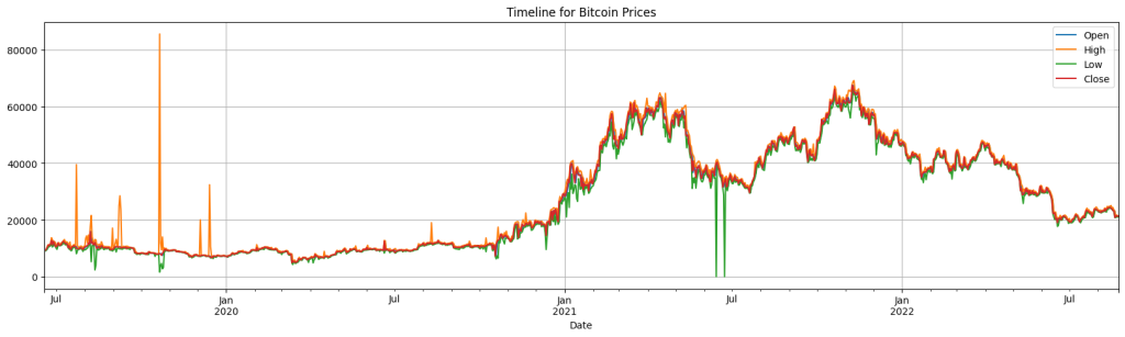
- The timeline above reveals more information about the dataset. Even though the descriptive stats and the boxplots before did not show such outliers, here we can see some extreme outliers for ‘High’ and ‘Low’ columns.
- This is another sign that shows how volatile cryptocurrencies (and stock markets as well) can be that makes it harder to build a solid ML model to predict valid outcomes.
- Previous stats did not reveal this information because it took all data points as a whole, rather than some fractions of a time line.
# Plot Bitcoin volume over time
df_btc.plot(x='Date', y=['Volume'],
            figsize=(20, 5), grid=True,
            title='Bitcoin Volume over time')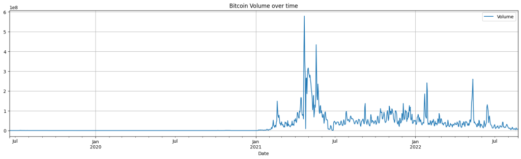
- Bitcoin volume over time shows high volatility as well. Let’s check those zero values.
# Check the zero volume observations
zero_volume_btc = df_btc[df_btc['Volume'] == 0]
zero_volume_btc| Date | Open | High | Low | Close | Volume | |
|---|---|---|---|---|---|---|
| 551 | 2020-12-20 | 20032.421875 | 24315.615234 | 19427.007812 | 23410.105469 | 0.0 |
| 552 | 2020-12-21 | 23408.089844 | 24261.000000 | 21757.462891 | 22036.162109 | 0.0 |
| 555 | 2020-12-24 | 22942.250000 | 23980.751953 | 20083.648438 | 20245.173828 | 0.0 |
- This looks odd, since we have ‘varying’ opening and closing prices but no volume for those days. Maybe there was some regulation issues.
- I double-checked the historic records of BTCB from earlier-mentioned platforms. They also reflect the same information.
▶ Handling Outliers:
- The above steps show the volatile character of cryptocurrencies, making it hard to handle outliers.
- Removing or adjusting outliers in a time series set may improve ML algorithms, however this way they would be prone to overfitting as well.
- Those outliers are an important part of a crypto-world and also of a stock-market analysis. They require deeper investigation, possibly involving bigger scale market research. For the simplicity of this study, I’ll keep them as they are.
3.4 Data Preprocessing
Target Variable
- Defining the target variable depends on the business goal. For this case, I needed to check the assignment paper. In the paper it is stated as “Define the target variable as the future Bitcoin prices (e.g., closing price in the next time window)“.
- Target variable will be the closing price, however the term ‘next time window’ and the point where and when we take the inputs to predict the outcome is not clear.
- We could take the current day’s opening price or some days earlier values and we could try to predict that given day’s closing price or some closing values ahead a time, e.g., predictions for the upcoming days or week.
- For these scenarios we will need different approaches. Considering the given information, I’ll consider using the model at the moment where we get the information of the opening price, and the target variable would be the closing price of that given day. Meaning that the models can not see the given days’ price values, except the opening price.
Feature Engineering
As we see above with the descriptive statistics and the graphs of the distributions, the prices and the volume are quite volatile and it will be hard to predict the outcome with the existing columns. Below I’ll check different approaches and create some new columns based on the existing ones.
Patterns within each Month
Let’s check if there are some patterns for some specific months or not.
# Create a new 'Month' column
df_btc['Month'] = df_btc['Date'].dt.month
# Create a new 'Month_txt' column
df_btc['Month_txt'] = df_btc['Date'].dt.month_name().str.slice(stop=3)
# Display the new columns
df_btc.head(3)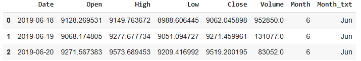
# Check Close and Volume averages for each month
df_btc_month = df_btc.groupby(['Month', 'Month_txt'], as_index=False)[['Close', 'Volume']].mean().sort_values('Month')
# without as_index=False, it returns a Series rather than Dataframe
df_btc_month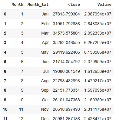
Looks like they differ per month, let’s visualize them to better grasp.
# Plot average Close prices per month
plt.bar(x=df_btc_month['Month_txt'], height=df_btc_month['Close'])
plt.plot()
plt.axhline(y=df_btc['Close'].mean(), linestyle="dashed", color='red', alpha=0.6, label="Average of all")
plt.xlabel("Months")
plt.ylabel("Average price in USD")
plt.title("Average Close Prices of Bitcoin per month")
plt.legend()
plt.show()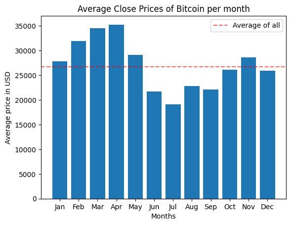
# Plot average Volume per month
plt.bar(x=df_btc_month['Month_txt'], height=df_btc_month['Volume'])
plt.plot()
plt.axhline(y=df_btc['Volume'].mean(), linestyle="dashed", color='red', alpha=0.6, label="Average of all")
plt.xlabel("Months")
plt.ylabel("Average volume in USD")
plt.title("Average Volume of Bitcoin per month")
plt.legend()
plt.show()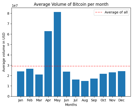
While above graph shows that April and May has the highest volume among all months, we can’t say this is valid for each year. Because our previous time-line plot revealed huge peaks during this months of 2021. They are skewing the distribution towards these months more. This might be also the explanation for those high values of Close price during this period of year.
In addition, around-3-year period is also not a long time to consider for monthly characteristics, especially when we have so much fluctuating movements. Therefore I won’t consider month column as a feature.
Patterns within Weekdays
Let’s check the same for weekdays as well.
# Create a new 'Weekday' column
df_btc['Weekday'] = df_btc['Date'].dt.day_name()
# Display the new column
df_btc.head(3)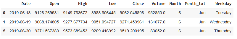
# Plot average Close and Volume per Weekday
df_btc_weekday = df_btc[['Weekday', 'Close', 'Volume']].groupby(['Weekday']).mean()
df_btc_weekday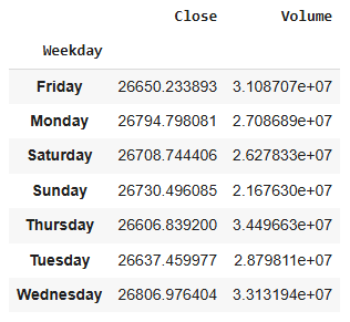
# Define order of days for the plot
weekday_order = ['Monday','Tuesday', 'Wednesday', 'Thursday','Friday','Saturday','Sunday']

# Create boxplots of average Close price (of Bitcoin) for each weekday
g = sns.boxplot(data = df_btc,
                y = 'Weekday',
                x =  'Close',
                order = weekday_order,
                showfliers = False)
g.set_title('Distribution of Bitcoin Close prices per weekday')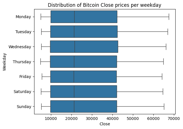
Unlike the traditional stock markets, cryptocurrencies can be bought everyday as seen above. The plotted distributions show only very little difference between weekdays for Bitcoin Close prices within the given time period.
# Create boxplots of Bitcoin Volume for each weekday
g = sns.boxplot(data = df_btc,
                y = 'Weekday',
                x =  'Volume',
                order = weekday_order,
                showfliers = False)
g.set_title('Distribution of Bitcoin Volume per weekday')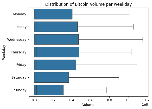
When we check the distributions of Bitcoin Volume per weekday, it seems the patterns vary a bit compared to each other. However it is not satisfactory to tell (Volume’s distribution per) weekdays can be a feature to consider, for mainly two reasons:
- Those differences are shown themselves only on the upper part of the data. The median and the distribution on the lower part of the data seem quite similar.
- When we add outliers to the distributions, those differences are scaled down quite much.
- For these reasons, I’ll drop month and day columns
# Drop Month and Weekdays columns
df_btc = df_btc.drop(columns=['Month', 'Month_txt', 'Weekday'])
Open and Close to be the Highest or the Lowest
Let’s check how many time we have an opening or closing price being the highest or lowest of that given day.
# Check High and Low points to happen exactly at the Opening or Closing for Bitcoin
btc_oc_hl = df_btc[(df_btc['Open'] == df_btc['Low']) | (df_btc['Open'] == df_btc['High']) |
                   (df_btc['Close'] == df_btc['Low']) | (df_btc['Close'] == df_btc['High'])]
print(len(btc_oc_hl))
print(round(len(btc_oc_hl)/len(df_btc), 2))
69 0.06
For Bitcoin dataset those instances are quite rare. We can’t consider them.
Higher, Lower or Equal Opening
Let’s check the distributions of the situations where the opening prices are higher or lower than the previous day’s closing price.
# Check higher Open than previous day's Close for Bitcoin
higher_start_btc = df_btc[df_btc['Open'] > df_btc['Close'].shift(1)]
print('Bitcoin data set:')
print('Higher Open:', len(higher_start_btc), 'that is', round(len(higher_start_btc)/len(df_btc)*100, 2), '%')

# Check equal Open compared to previous day's Close for Bitcoin
equal_start_btc = df_btc[df_btc['Open'] == df_btc['Close'].shift(1)]
print('Equal Open:', len(equal_start_btc), 'that is', round(len(equal_start_btc)/len(df_btc)*100, 2), '%')

# Check lower Open than previous day's Close for Bitcoin
lower_start_btc = df_btc[df_btc['Open'] < df_btc['Close'].shift(1)]
print('Lower Open:', len(lower_start_btc), 'that is', round(len(lower_start_btc)/len(df_btc)*100, 2), '%')
Bitcoin data set:
Higher Open: 468 that is 40.24 %
Equal Open: 242 that is 20.81 %
Lower Open: 452 that is 38.87 %
The distributions are promising, we can try them as features. Let’s create new columns to reflect these. Some things to note:
- When we check previous day’s closing value by using .shift(1), the very first day won’t get any value because there is no previous day for it. We need to take care of that.
- Let’s compare these differences (of the current day’s Open and previous day’s Close) relative to the previous day’s Close too. This way we will have some idea about the power of those changes as well.
- But we will need to choose only one of these two new columns for a model, since they will be highly correlated with each other.
# Check the first statement above
len(df_btc) - len(higher_start_btc) - len(equal_start_btc) - len(lower_start_btc)
1
# Create the 'Change' column with conditions, assign NaN as 0
df_btc['Change'] = np.select(
    [
        df_btc['Open'] < df_btc['Close'].shift(1),  # Condition for 'lower'
        df_btc['Open'] > df_btc['Close'].shift(1),  # Condition for 'higher'
        df_btc['Open'] == df_btc['Close'].shift(1)  # Condition for 'equal'
    ],
    [
        -1,  # 'lower'
        1,   # 'higher'
        0    # 'equal'
    ],
    default = 0  # If no condition matches, default to 0 instead of NaN
)

# Calculate the percentage change relative to the previous day's closing price
df_btc['Change_perc'] = round(((df_btc['Open'] - df_btc['Close'].shift(1)) / df_btc['Close'].shift(1)) * 100, 3)

# Fill NaN in 'Change_perc' with 0 (since the first row has no previous close)
df_btc['Change_perc'] = df_btc['Change_perc'].fillna(0)df_btc.head()| Date | Open | High | Low | Close | Volume | Change | Change_perc | |
|---|---|---|---|---|---|---|---|---|
| 0 | 2019-06-18 | 9128.269531 | 9149.763672 | 8988.606445 | 9062.045898 | 952850.0 | 0 | 0.000 |
| 1 | 2019-06-19 | 9068.174805 | 9277.677734 | 9051.094727 | 9271.459961 | 131077.0 | 1 | 0.068 |
| 2 | 2019-06-20 | 9271.567383 | 9573.689453 | 9209.416992 | 9519.200195 | 83052.0 | 1 | 0.001 |
| 3 | 2019-06-21 | 9526.833984 | 10130.935547 | 9526.833984 | 10127.998047 | 76227.0 | 1 | 0.080 |
| 4 | 2019-06-22 | 10151.890625 | 11171.013672 | 10083.189453 | 10719.981445 | 84485.0 | 1 | 0.236 |
High and Low: ‘H-L Average over Open’ & ‘H-L Variance over O-C Variance’
Let’s consider the highest and lowest prices as well. But remember, we can’t use the current day’s values. Different new values can be created but I’ll focus on two of them:
- The average of previous day’s highest and lowest prices over current day’s opening price.
- The difference of previous day’s highest and lowest prices over the difference of current day’s opening price and previous day’s closing price.
With these, I intend to get some insights, particularly for identifying market states and predicting trend continuation. Because the price range part captures volatility over the period, and the price gap part captures momentum.
# Calculate the ratio of previous day's High and Low average over Open
df_btc['HL_avg_to_Open'] = round((df_btc['High'].shift(1) + df_btc['Low'].shift(1)) / 2 / df_btc['Open'] ,3)

# Calculate the ratio of previous day's High and Low difference over the Open and previous day's Close difference
df_btc['HL_dif_to_OC_dif'] = round((df_btc['High'].shift(1) - df_btc['Low'].shift(1)) / (df_btc['Open'] - df_btc['Close'].shift(1)) ,3)
These new columns will also have NaNs on the first row. This will repeat on upcoming steps with other newly-created columns too. We may have infinity values as well, caused by division by zero. For both situations, I’ll fullfill them with zero, to handle some errors (such as arrays must not contain infs and NaNs) that may cause during some computations like correlations.
▶ We will need to do some scaling these new columns, since they are already showing up in different scales.
Last 7 Days: Close & Volume
- Until now I was checking the relationship of current values with only the previous day’s values. Let’s expend it to a week, focusing on Close and Volume.
- The volume has large amounts, so better to compress it with log transformation, even before doing scaling for all.
# Calculate last 7 day's average of Close
df_btc['Close_7_day_avg'] = df_btc['Close'].shift(1).rolling(window=7).mean()
# .shift(1) not to include the current day

# Calculate last 7 day's average of Volume
df_btc['Vol_7_day_avg'] = df_btc['Volume'].shift(1).rolling(window=7).mean()

# Apply log transformation to the 7-day average Volume
df_btc['Log_Vol_7_day_avg'] = np.log(df_btc['Vol_7_day_avg'] + 1)  # +1 to avoid log(0)
Price Prediction in the Crypto-market: SMA, EMA, RSI
- At this point, I need to extend my methods by doing some research. In fact, the steps taken above include some of them. Using past values as predictors (e.g., closing price of the previous day, week) is called Lagged Features and I’ve already implied such.
- The accuracy of price prediction in the cryptocurrency market can be improved by using technical indicators such as the SMA, EMA, and RSI as input. Introduction the SMA and EMA are trend-following indicators that are used to amplify price data and pinpoint the trend’s direction. The momentum oscillator RSI, on the other hand, gauges how strongly prices fluctuate.
- The Simple Moving Average (SMA) is the arithmetic mean of a dataset over a specific number of periods. It’s called “simple” because all values in the period have equal weight. In fact, this is what I did above while calculating the last 7 days averages for Close and Volume.
- SMA is slow to respond to changes because it gives equal weight to all data points in the period. Exponential Moving Average (EMA), on the other side, exponentially decreasing weights to older prices. We can use it again for the last 7 days, but this time it will give more weight to recent days, introducing different information than SMA.
- The Relative Strength Index (RSI) is a momentum oscillator used to measure the speed and change of price movements. It helps identify overbought or oversold conditions in the market, which can signal potential reversals or confirm trends. Since RSI takes into consideration both gains and losses at the same time, we can take a 14-days period to calculate them.
To perform above mentioned calculations Python’s Technical Analysis Library (Talib) is imported.
# Install talib to calculate EMA, SMA and RFI
url = 'https://anaconda.org/conda-forge/libta-lib/0.4.0/download/linux-64/libta-lib-0.4.0-h166bdaf_1.tar.bz2'
!curl -L $url | tar xj -C /usr/lib/x86_64-linux-gnu/ lib --strip-components=1
url = 'https://anaconda.org/conda-forge/ta-lib/0.4.19/download/linux-64/ta-lib-0.4.19-py310hde88566_4.tar.bz2'
!curl -L $url | tar xj -C /usr/local/lib/python3.10/dist-packages/ lib/python3.10/site-packages/talib --strip-components=3
import talib# Compute SMA for Close and Volume
df_btc['SMA_7_Close'] = talib.SMA(df_btc['Close'].shift(1), 7)
df_btc['SMA_7_Volume'] = talib.SMA(df_btc['Volume'].shift(1), 7)
df_btc['SMA_7_Vol_log'] = np.log(df_btc['SMA_7_Volume'] + 1)
# Compute EMA for Close and Volume
df_btc['EMA_7_Close'] = talib.EMA(df_btc['Close'].shift(1), 7)
df_btc['EMA_7_Volume'] = talib.EMA(df_btc['Volume'].shift(1), 7)
df_btc['EMA_7_Vol_log'] = np.log(df_btc['EMA_7_Volume'] + 1)
# Compute RSI for Close and Volume
df_btc['RSI_14_Close'] = talib.RSI(df_btc['Close'].shift(1), 14)
df_btc['RSI_14_Volume'] = talib.RSI(df_btc['Volume'].shift(1), 14)# Compare initial calculation with the ones coming from talib
to_compare = df_btc[['Close_7_day_avg', 'Vol_7_day_avg', 'Log_Vol_7_day_avg', 'SMA_7_Close', 'SMA_7_Volume', 'SMA_7_Vol_log']]
# Check the comparison
to_compare.tail(10)| Close_7_day_avg | Vol_7_day_avg | Log_Vol_7_day_avg | SMA_7_Close | SMA_7_Volume | SMA_7_Vol_log | |
|---|---|---|---|---|---|---|
| 1153 | 23838.373605 | 9.480461e+06 | 16.064744 | 23838.373605 | 9.480461e+06 | 16.064744 |
| 1154 | 23999.602400 | 9.667308e+06 | 16.084261 | 23999.602400 | 9.667308e+06 | 16.084261 |
| 1155 | 24043.323103 | 9.804977e+06 | 16.098401 | 24043.323103 | 9.804977e+06 | 16.098401 |
| 1156 | 24144.000558 | 9.652858e+06 | 16.082765 | 24144.000558 | 9.652858e+06 | 16.082765 |
| 1157 | 24057.962333 | 8.275720e+06 | 15.928837 | 24057.962333 | 8.275720e+06 | 15.928837 |
| 1158 | 23950.169922 | 6.937017e+06 | 15.752383 | 23950.169922 | 6.937017e+06 | 15.752383 |
| 1159 | 23453.934152 | 7.905015e+06 | 15.883008 | 23453.934152 | 7.905015e+06 | 15.883008 |
| 1160 | 22988.511161 | 7.940757e+06 | 15.887519 | 22988.511161 | 7.940757e+06 | 15.887519 |
| 1161 | 22596.575893 | 7.991712e+06 | 15.893916 | 22596.575893 | 7.991712e+06 | 15.893916 |
| 1162 | 22195.934964 | 7.528807e+06 | 15.834247 | 22195.934964 | 7.528807e+06 | 15.834247 |
Since we are sure these above values are the same, we can drop the initial calculations.
# Drop repeating columns
df_btc = df_btc.drop(['Close_7_day_avg', 'Vol_7_day_avg', 'Log_Vol_7_day_avg'], axis=1)
3.5 Organize Columns
It’s time to tidy up a little bit the dataframe.
Infinity & NaN
- Let’s check divisions by zero that results as inf and then fulfill them with zero.
- I’ll fulfill NaNs with zero as well, not to have array-based value errors in the following computations.
# Check inf values
inf_count_by_column = np.sum(np.isinf(df_btc.select_dtypes(include=[np.number])))

print("Number of inf values per column:")
print(inf_count_by_column)
Number of inf values per column:
Open 0
High 0
Low 0
Close 0
Volume 0
Status 0
Change 0
Change_perc 0
HL_avg_to_Open 0
HL_dif_to_OC_dif 242
SMA_7_Close 0
SMA_7_Volume 0
SMA_7_Vol_log 0
EMA_7_Close 0
EMA_7_Volume 0
EMA_7_Vol_log 0
RSI_14_Close 0
RSI_14_Volume 0
dtype: int64
# Replace inf with zero
df_btc['HL_dif_to_OC_dif'] = df_btc['HL_dif_to_OC_dif'].replace([np.inf, -np.inf], 0)
# Fulfill NaNs with zero
df_btc = df_btc.fillna(0)Keep log-version of Volume and Rename Columns
- Choosing SMA or EMA will be done during the selection phase. But I’ll drop the SMA and EMA of Volume, since I’ll be using the log version of those.
- I’ll rename some columns for better usage: HL_avg_to_Open –> Momentum, HL_dif_to_OC_dif –> V_to_L (as in Volatility over Momentum)
# Drop columns
df_btc = df_btc.drop(['SMA_7_Volume', 'EMA_7_Volume'], axis=1)
# Change the column names
df_btc.rename(columns={'HL_avg_to_Open': 'Momentum', 'HL_dif_to_OC_dif': 'V_to_L'}, inplace=True)
# Check the changes
df_btc.head(3)| Date | Open | High | Low | Close | Volume | Change | Change_perc | Momentum | V_to_L | SMA_7_Close | SMA_7_Vol_log | EMA_7_Close | EMA_7_Vol_log | RSI_14_Close | RSI_14_Volume | |
|---|---|---|---|---|---|---|---|---|---|---|---|---|---|---|---|---|
| 0 | 2019-06-18 | 9128.269531 | 9149.763672 | 8988.606445 | 9062.045898 | 952850.0 | 0 | 0.000 | 0.000 | 0.000 | 0.0 | 0.0 | 0.0 | 0.0 | 0.0 | 0.0 |
| 1 | 2019-06-19 | 9068.174805 | 9277.677734 | 9051.094727 | 9271.459961 | 131077.0 | 1 | 0.068 | 1.000 | 26.295 | 0.0 | 0.0 | 0.0 | 0.0 | 0.0 | 0.0 |
| 2 | 2019-06-20 | 9271.567383 | 9573.689453 | 9209.416992 | 9519.200195 | 83052.0 | 1 | 0.001 | 0.988 | 2109.282 | 0.0 | 0.0 | 0.0 | 0.0 | 0.0 | 0.0 |
4 Feature Selection
4.1 Initial Feature Selection: Correlation
plt.figure(figsize=(10, 8))
df_btc_study = df_btc.filter(['Close', 'Status', 'Change',
       'Change_perc', 'Momentum', 'V_to_L', 'SMA_7_Close', 'SMA_7_Vol_log',
       'EMA_7_Close', 'EMA_7_Vol_log', 'RSI_14_Close', 'RSI_14_Volume'], axis=1)

corr_study = df_btc_study.corr()

sns.heatmap(corr_study, annot=True, cmap='coolwarm', square=True, fmt=".3f")
plt.title('Correlation Matrix')
plt.show()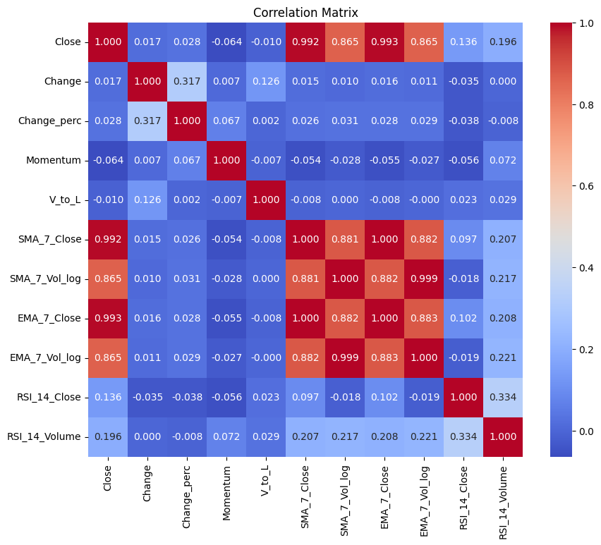
▶ As mentioned earlier, SMA and EMA are highly correlated with each other simply because they are both based on the same calculation. We’ll need to choose one of them when fitting the model not to lead to redundancy. We should also note that Pearson correlation measures the linear relationship between variables. Low values in the above correlation matrix might be due to a non-linear relationship.
4.2 Split the Data
For time series data, random splitting is not suitable because it breaks the temporal order of the data, which is critical for preserving the relationship between past and future. Instead, we need to use methods that respect the time-dependent nature of the data.
The data was sorted by date earlier, so I’ll take the first 80% of that order as a training set.
# Time-Based Train-Test Split (e.g., 80% train, 20% test)
train_size = int(len(df_btc) * 0.8)
train_data = df_btc[:train_size]
test_data = df_btc[train_size:]
I’ll have two main sets of features:
- The first one (‘features’) will hold all newly created columns. This will be the base set for KNN and Random Forest. Then a feature selection will be implied based on their importance score. Finally the models will be fitted with both sets to be able to compare them.
- The second one (‘features_reg’) will hold all newly created columns, except the SMAs. This will be the base set for Linear Regression. Then a feature selection will be implied based on mean squared error calculation. Finally the model will be fitted with both sets to be able to compare them.
# Separate features and targets
features = ['Change', 'Change_perc', 'Momentum', 'V_to_L', 'SMA_7_Close', 'SMA_7_Vol_log',
       'EMA_7_Close', 'EMA_7_Vol_log', 'RSI_14_Close', 'RSI_14_Volume']

features_reg = ['Change', 'Change_perc', 'Momentum', 'V_to_L', 'EMA_7_Close',
                'EMA_7_Vol_log', 'RSI_14_Close', 'RSI_14_Volume']

X_train = train_data[features]
y_train_close = train_data['Close']

X_test = test_data[features]
y_test_close = test_data['Close']

X_train_reg = train_data[features_reg]
X_test_reg = test_data[features_reg]
# Print the sizes of train and test sets
print(f"Training set: {X_train.shape}, Testing set: {X_test.shape}")Training set: (930, 10), Testing set: (233, 10)
4.3 Scale the Data
I’ll apply scaling techniques to standardize features for scaling-sensitive methods:
Standardization (Z-Score Scaling): For methods (here Linear Regression) that assume a normal distribution.
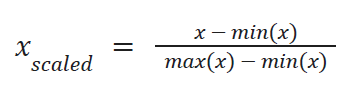
Normalization (Min-Max Scaling): For methods (here KNN) sensitive to feature ranges.
Tree-based models split data based on feature thresholds, so they are scale-invariant.
from sklearn.preprocessing import StandardScaler, MinMaxScaler# Standardization for regression models
scaler = StandardScaler()
X_train_scaled= scaler.fit_transform(X_train_reg)
X_test_scaled = scaler.transform(X_test_reg)
# Normalization for KNN
normalizer = MinMaxScaler()
X_train_normalized = normalizer.fit_transform(X_train)
X_test_normalized = normalizer.transform(X_test)
# Tree-based models (no scaling required)
X_train_tree = X_train.copy()
X_test_tree = X_test.copy()4.4 Feature Selection: RFE
Basic methods (e.g., correlation) may overlook interactions between features, therefore advanced feature selection methods can help us to handle high-dimensional datasets. These methods aim to identify the most predictive features while considering interactions, redundancy, and model-specific needs.
I’ll perform Recursive Feature Elimination (RFE), that starts with all features and recursively eliminates the least important ones, retraining the model each time, to identify the optimal subset.
4.4.1 Linear Regression
from sklearn.feature_selection import RFECV
from sklearn.model_selection import TimeSeriesSplit

from sklearn.linear_model import LinearRegression
# TimeSeriesSplit
tscv = TimeSeriesSplit(n_splits=5)
# For 'Close' target (Linear Regression)
lr_model = LinearRegression()
rfe_close = RFECV(estimator=lr_model, step=1, cv=tscv, scoring='neg_mean_squared_error')
rfe_close.fit(X_train_scaled, y_train_close)
selected_features_close = X_train_reg.columns[rfe_close.support_]
print(f"Selected features for 'Close': {selected_features_close}")Selected features for 'Close': Index(['EMA_7_Close', 'EMA_7_Vol_log', 'RSI_14_Close', 'RSI_14_Volume'], dtype='object')
Calculated by mean squared error, RFE selected features for Linear Regression are: ‘EMA_7_Close’, ‘EMA_7_Vol_log’, ‘RSI_14_Close’, ‘RSI_14_Volume’. I’ll create a subset with these features:
# Transform datasets based on selected features
X_train_close_rfe = X_train_scaled[:, rfe_close.support_]
X_test_close_rfe = X_test_scaled[:, rfe_close.support_]
4.4.2 Random Forest Regressor
from sklearn.ensemble import RandomForestRegressor# Random Forest Regressor for 'Close' (Continuous Target)
rf_reg = RandomForestRegressor(n_estimators=100, random_state=42)
rf_reg.fit(X_train_tree, y_train_close)
feature_importances_close = rf_reg.feature_importances_
# Combine Feature Importance into DataFrames
features = X_train.columns
importance_df_close = pd.DataFrame({
'Feature': features,
'Importance_Close': feature_importances_close
}).sort_values(by='Importance_Close', ascending=False)
print("Top Features for 'Close':")
print(importance_df_close.head())Top Features for 'Close':
Feature Importance_Close
6 EMA_7_Close 0.559815
4 SMA_7_Close 0.430999
8 RSI_14_Close 0.003829
5 SMA_7_Vol_log 0.001567
7 EMA_7_Vol_log 0.000914
Top five features for Close by their importance score are listed above. Even though apart from the EMA and SMA of Close price, the scores of other features are quite low, I’ll consider these five features as another subset. Because Volume in crypto market plays a crucial role.
features_rf_reg = ['SMA_7_Close', 'SMA_7_Vol_log', 'EMA_7_Close', 'EMA_7_Vol_log', 'RSI_14_Close']

X_train_rf_reg = train_data[features_rf_reg]
X_test_rf_reg = test_data[features_rf_reg]
4.4.3 KNN Regression
from sklearn.neighbors import KNeighborsRegressor
from scipy.stats import pearsonr
# Initialize an empty list to store correlation results
correlation_results = []
# Calculate correlations for each feature
for col in X_train.columns:
# Pearson correlation for 'Close'
corr_close, pval_close = pearsonr(X_train[col], y_train_close)
# Append results as a dictionary
correlation_results.append({
'Feature': col,
'Correlation_Close': corr_close,
'PValue_Close': pval_close,
})
# Convert the list of dictionaries into a DataFrame
correlation_with_target = pd.DataFrame(correlation_results)
correlation_with_target| Feature | Correlation_Close | PValue_Close | |
|---|---|---|---|
| 0 | Change | 0.021665 | 5.093319e-01 |
| 1 | Change_perc | 0.032375 | 3.240185e-01 |
| 2 | Momentum | -0.063084 | 5.446534e-02 |
| 3 | V_to_L | -0.021892 | 5.048996e-01 |
| 4 | SMA_7_Close | 0.992835 | 0.000000e+00 |
| 5 | SMA_7_Vol_log | 0.908133 | 0.000000e+00 |
| 6 | EMA_7_Close | 0.993985 | 0.000000e+00 |
| 7 | EMA_7_Vol_log | 0.908290 | 0.000000e+00 |
| 8 | RSI_14_Close | 0.181783 | 2.367402e-08 |
| 9 | RSI_14_Volume | 0.210607 | 8.761178e-11 |
Based on Pearson correlation calculation, the features’ correlation rates with Close prize and their p-value are printed above. I filter them below based on threshold to create another subset with them.
# Filter features based on thresholds
selected_features_close = correlation_with_target.loc[
    (correlation_with_target['Correlation_Close'].abs() > 0.1) &
    (correlation_with_target['PValue_Close'] < 0.05),
    'Feature'
]

print("Selected Features for 'Close':", list(selected_features_close))
Selected Features for 'Close': ['SMA_7_Close', 'SMA_7_Vol_log', 'EMA_7_Close', 'EMA_7_Vol_log', 'RSI_14_Close', 'RSI_14_Volume']
To handle multicollinearity I keep EMA in the subset, but remove SMA out.
features_knn = ['EMA_7_Close', 'EMA_7_Vol_log', 'RSI_14_Close', 'RSI_14_Volume']# Create subsets with selected features
X_train_knn = train_data[features_knn]
X_test_knn = test_data[features_knn]
# Scale features for both targets
X_train_knn_scaled = pd.DataFrame(normalizer.fit_transform(X_train[features_knn]), columns=features_knn)
X_test_knn_scaled = pd.DataFrame(normalizer.transform(X_test[features_knn]), columns=features_knn)5 Model Training and Evaluation
Three different models (Random Forest, Regression, and KNN) will be implemented for Bitcoin price prediction. For each model, two different sets of features will be used, that are defined above.
from sklearn.metrics import mean_squared_error, accuracy_score, r2_score
from sklearn.metrics import confusion_matrix, ConfusionMatrixDisplay
from sklearn.metrics import classification_report, roc_auc_score
5.1 Linear Regression
Model 1a:
features_reg = [‘Change’, ‘Change_perc’, ‘Momentum’, ‘V_to_L’, ‘EMA_7_Close’, ‘EMA_7_Vol_log’, ‘RSI_14_Close’, ‘RSI_14_Volume’]
# Linear Regression for 'Close'
lr_model.fit(X_train_reg, y_train_close)
y_pred_LinReg_a = lr_model.predict(X_test_reg)

# Compute MSE
mse_close = mean_squared_error(y_test_close, y_pred_LinReg_a)
# Compute RMSE
model_rmse = np.sqrt(mse_close)
# Compute R²
r2 = r2_score(y_test_close, y_pred_LinReg_a)

# Print results
print(f"Linear Regression MSE: {mse_close:.2f}")
print(f"Linear Regression RMSE: {model_rmse:.2f}")
print(f"Linear Regression R²: {r2:.2f}")
Linear Regression MSE: 2669453.94
Linear Regression RMSE: 1633.85
Linear Regression R²: 0.97
R2 score looks high, however we need to be sure that the residuals show no patterns:
# Compute Residuals
residuals = y_test_close - y_pred_LinReg_a

# Plot Residuals
plt.figure(figsize=(6, 4))
plt.scatter(range(len(residuals)), residuals, alpha=0.6, edgecolors="k", label="Residuals")
plt.axhline(0, color="red", linestyle="--", label="Zero Error Line")
plt.title("Residuals of Linear Regression Model")
plt.xlabel("Observation Index")
plt.ylabel("Residual (Actual - Predicted)")
plt.legend()
plt.tight_layout()
plt.show()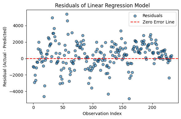
Residuals don’t seem to scatter randomly around zero error line. Residual plot indeed has a pattern, especially where dots overlap each other, like a zig-zag shape reflecting the fluctuating movements of the prices. Therefore we can’t tell the homoscedasticity assumption is met.
Model 1b:
X_train_close_rfe = [‘EMA_7_Close’, ‘EMA_7_Vol_log’, ‘RSI_14_Close’, ‘RSI_14_Volume’]
# Linear Regression for 'Close'
lr_model.fit(X_train_close_rfe, y_train_close)
y_pred_LinReg_b = lr_model.predict(X_test_close_rfe)

# Compute MSE
mse_close = mean_squared_error(y_test_close, y_pred_LinReg_b)
# Compute RMSE
model_rmse = np.sqrt(mse_close)
# Compute R²
r2 = r2_score(y_test_close, y_pred_LinReg_b)

# Print results
print(f"Linear Regression MSE: {mse_close:.2f}")
print(f"Linear Regression RMSE: {model_rmse:.2f}")
print(f"Linear Regression R²: {r2:.2f}")
Linear Regression MSE: 2677830.30
Linear Regression RMSE: 1636.41
Linear Regression R²: 0.97
Root Mean Squared Error (RMSE) of Linear Regression with limited features (1636.41) doesn’t show any improvement compared to the initial set of features (1633.85).
5.2 Random Forest Regressor
Model 2a:
features = [‘Change’, ‘Change_perc’, ‘Momentum’, ‘V_to_L’, ‘SMA_7_Close’, ‘SMA_7_Vol_log’, ‘EMA_7_Close’, ‘EMA_7_Vol_log’, ‘RSI_14_Close’, ‘RSI_14_Volume’]
# Train Random Forest Regressor
rf_reg = RandomForestRegressor(n_estimators=100, random_state=42)
rf_reg.fit(X_train_tree, y_train_close)

# Predictions
y_pred_RanFor_a = rf_reg.predict(X_test_tree)
# Evaluate Regression Performance
mse_close_rf = mean_squared_error(y_test_close, y_pred_RanFor_a)
rmse_close_rf = np.sqrt(mse_close_rf)
r2_close_rf = r2_score(y_test_close, y_pred_RanFor_a)
print(f"Random Forest Regression MSE: {mse_close_rf:.2f}")
print(f"Random Forest Regression RMSE: {rmse_close_rf:.2f}")
print(f"Random Forest Regression R²: {r2_close_rf:.2f}")Random Forest Regression MSE: 8349162.74
Random Forest Regression RMSE: 2889.49
Random Forest Regression R²: 0.90
Both RMSE and R2 scores of Random Forest with the initial set of features performed worse than Linear Regression.
Model 2b:
features_rf_reg = [‘SMA_7_Close’, ‘SMA_7_Vol_log’, ‘EMA_7_Close’, ‘EMA_7_Vol_log’, ‘RSI_14_Close’]
# Train Random Forest Regressor
rf_reg.fit(X_train_rf_reg, y_train_close)

# Predictions
y_pred_RanFor_b = rf_reg.predict(X_test_rf_reg)
# Evaluate Regression Performance
mse_close_rf = mean_squared_error(y_test_close, y_pred_RanFor_b)
rmse_close_rf = np.sqrt(mse_close_rf)
r2_close_rf = r2_score(y_test_close, y_pred_RanFor_b)
print(f"Random Forest Regression MSE: {mse_close_rf:.2f}")
print(f"Random Forest Regression RMSE: {rmse_close_rf:.2f}")
print(f"Random Forest Regression R²: {r2_close_rf:.2f}")Random Forest Regression MSE: 7595475.41
Random Forest Regression RMSE: 2755.99
Random Forest Regression R²: 0.90
Root Mean Squared Error (RMSE) of Random Forest with limited features (2755.99) show slight improvement compared to the initial set of features (2889.49). However both versions perform worse than Linear Regression.
5.3 KNN Regression
Model 3a:
features = [‘Change’, ‘Change_perc’, ‘Momentum’, ‘V_to_L’, ‘SMA_7_Close’, ‘SMA_7_Vol_log’, ‘EMA_7_Close’, ‘EMA_7_Vol_log’, ‘RSI_14_Close’, ‘RSI_14_Volume’]
# Train KNN
knn_reg = KNeighborsRegressor(n_neighbors=5)
knn_reg.fit(X_train_normalized, y_train_close)

# Predictions
y_pred_Knn_a = knn_reg.predict(X_test_normalized)
# Evaluate Regression Performance
mse_close_knn = mean_squared_error(y_test_close, y_pred_Knn_a)
rmse_close_knn = np.sqrt(mse_close_rf)
r2_close_knn = r2_score(y_test_close, y_pred_Knn_a)
print(f"Random Forest Regression MSE: {mse_close_knn:.2f}")
print(f"Random Forest Regression RMSE: {rmse_close_knn:.2f}")
print(f"Random Forest Regression R²: {r2_close_knn:.2f}")Random Forest Regression MSE: 47252303.84
Random Forest Regression RMSE: 2755.99
Random Forest Regression R²: 0.41
Both RMSE and R2 scores of KNN with the initial set of features performed worse than Linear Regression and Random Forest.
Model 3b:
features_knn = [‘EMA_7_Close’, ‘EMA_7_Vol_log’, ‘RSI_14_Close’, ‘RSI_14_Volume’]
# Train KNN
knn_reg.fit(X_train_knn_scaled, y_train_close)

# Predictions
y_pred_Knn_b = knn_reg.predict(X_test_knn_scaled)
# Evaluate Regression Performance
mse_close_knn = mean_squared_error(y_test_close, y_pred_Knn_b)
rmse_close_knn = np.sqrt(mse_close_rf)
r2_close_knn = r2_score(y_test_close, y_pred_Knn_b)
print(f"Random Forest Regression MSE: {mse_close_knn:.2f}")
print(f"Random Forest Regression RMSE: {rmse_close_knn:.2f}")
print(f"Random Forest Regression R²: {r2_close_knn:.2f}")Random Forest Regression MSE: 48176489.06
Random Forest Regression RMSE: 2755.99
Random Forest Regression R²: 0.39
Root Mean Squared Error (RMSE) of KNN with limited features show no improvement compared to the initial set of features. And both versions perform worse than previous models.
5.4 Comparing the Models
Linear Regression with the least RMSE scores performed best compared to the Random Forest and KNN. However, plotted residuals revealed a biased pattern, that we can’t assume it’s a good predictor for a time series dataset like Bitcoin records here.
Plotting the actual and predicted values both on scatterplot and on a time-series graph might reveal different insights.
Actual vs Predicted: Scatter plot
# Visualize predictions for regression
def plot_regression_results(y_actual, y_pred, title="Regression Results"):
    plt.figure(figsize=(8, 6))
    plt.scatter(y_actual, y_pred, alpha=0.6, color="blue", label="Predictions")
    plt.plot([min(y_actual), max(y_actual)], [min(y_actual), max(y_actual)],
             color="red", linestyle="--", label="Perfect Prediction")
    plt.xlabel("Actual Values")
    plt.ylabel("Predicted Values")
    plt.title(title)
    plt.legend()
    plt.grid(True)
    plt.show()
# Plot actual vs predicted scatter plot for Linear Regression
plot_regression_results(y_test_close, y_pred_LinReg_a, title="Linear Regression: Close Price")# Plot actual vs predicted scatter plot for Random Forest
plot_regression_results(y_test_close, y_pred_RanFor_a, title="Random Forest: Close Price")# Plot actual vs predicted scatter plot for KNN
plot_regression_results(y_test_close, y_pred_Knn_a, title="KNN: Close Price")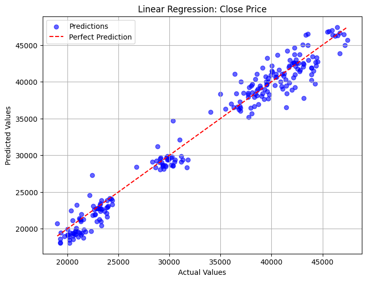
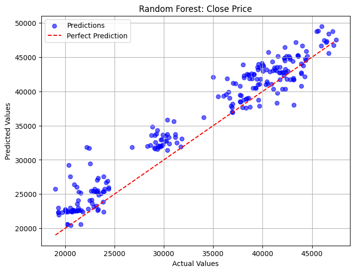
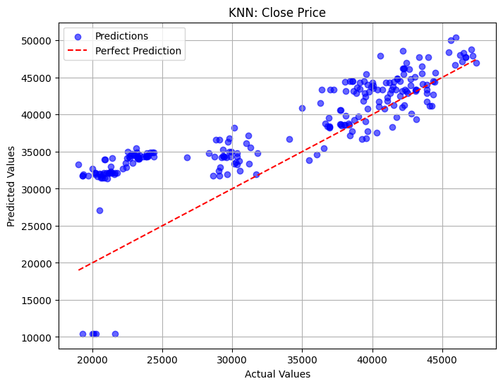
- Linear Regression’s predictions are closer to the ‘perfect prediction’ line compared to other models.
- Random Forest tends to over predict compared to Linear Regression.
- KNN’s predictions on lower values are highly overpredicted compared to other models.
- All models showed three clusters that needed further investigation.
To check these clusters, I’ll plot the histogram of the actual values (to see if these clusters exist there too) and compare the models’ predictions over it.
Actual vs Predicted: Histogram
# Histogram of Close prices
sns.histplot(y_train_close, kde=True, bins=50)
plt.title("Distribution of the Actual Close Prices")
plt.xlabel("Close Price")
plt.show()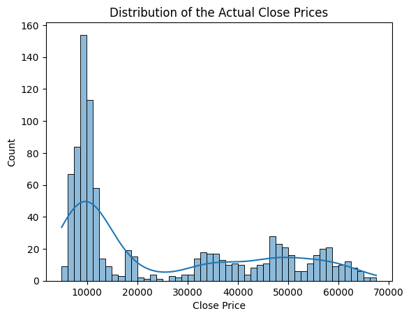
It seems that there are some clustering patterns within the distribution of Close prices. Let’s check how they relate with each prediction too.
actual_values = y_train_close
predicted_LinReg = y_pred_LinReg_a  # Predicted values from Linear Regression

# Create a histogram with overlaid KDE for both actual and predicted
plt.figure(figsize=(10, 6))

# Plot actual values
sns.histplot(actual_values, kde=True, color="blue", label="Actual", bins=100, stat="density", alpha=0.6)

# Plot predicted values
sns.histplot(predicted_LinReg, kde=True, color="orange", label="Predicted", bins=60, stat="density", alpha=0.6)

# Add title and legend
plt.title("Overlay of Actual and Predicted Values: Linear Regression", fontsize=14)
plt.xlabel("Close Price", fontsize=12)
plt.ylabel("Density", fontsize=12)
plt.legend(fontsize=12)

# Show the plot
plt.show()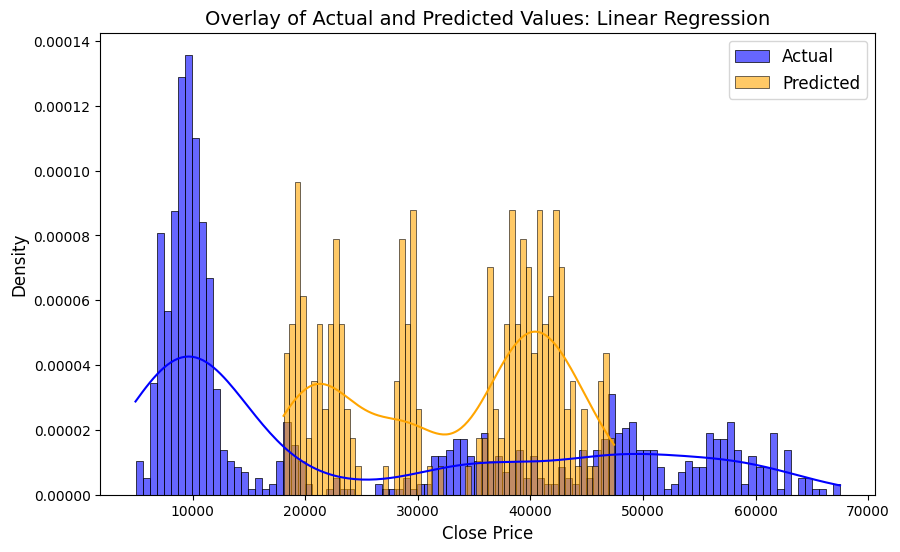

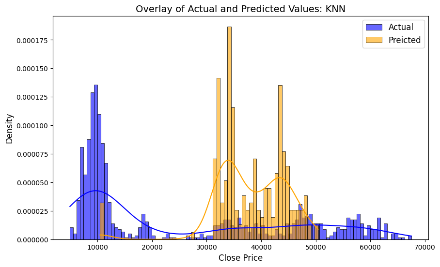
All models struggle to handle the volatile movements of Close price. While Linear Regression catches patterns better than other models, KNN’s predictions tend to cluster more towards the upper ranges of the prices.
Actual vs Predicted: Time-series Graph
Finally, I’ll observe the predictions on time-series graph to check how they react to the volatile character of the prices.
timestamps = df_btc['Date'].loc[X_test.index]

plt.figure(figsize=(20, 5))
plt.plot(timestamps, y_test_close, label="Actual Prices", color="red", linewidth=2)
plt.plot(timestamps, y_pred_LinReg_b, label="Linear Reg.", color="blue", linestyle="--", linewidth=2)
plt.plot(timestamps, y_pred_RanFor_b, label="Random For.", color="deepskyblue", linestyle="--", linewidth=2)
plt.plot(timestamps, y_pred_Knn_b, label="Knn", color="olive", linestyle="--", linewidth=2)

plt.xlabel("Time")
plt.ylabel("Bitcoin Price")
plt.title("Time-Series Plot with Limited Features")
plt.legend()
plt.grid(True)
plt.ylim(bottom=0) # Set y-axis starting from 0
plt.show()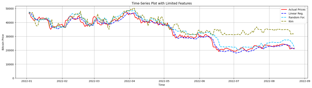
Even though the models follow similar patterns as with the actual price changes, we can’t be confident to say that these models can be used for an accurate prediction. Because the predicted lines don’t necessarily follow the correct direction nor in consistent proportions.
- The Linear Regression provides the smoothest line even the actual prices deviate. Meaning that it can’t ‘catch’ the vivid fluctuations quite well, due to its inability to capture complex patterns.
- Random Forest seems to be able to follow the up-and-down movements slightly better, most probably caused by handling non-linear relationships better. However it over-predicts compared to the Linear Regression.
- KNN over-predicts even greater than Random Forest and on the last part of the data (after mid-2022), it struggles even to follow general trends.
I’ll repeat the same plot with the initial set of features too to check the model’s performance change:
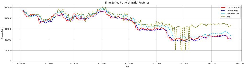
Plotting the predictions with the initial set of features highlights how feature selection and model dynamics influence models’ behavior, particularly KNN’s. KNN reflects sharp drops around July 2022. The initial feature set might include irrelevant or noisy features that don’t correlate well with the target. KNN can be sensitive to such features because it uses distances in the feature space to determine neighbors.
6 Going Forward
Takeaways
As demonstrated above, KNN does not account for temporal dynamics explicitly. Unlike random forests, which can capture interactions, or linear regression, which smooths trends, KNN operates strictly based on local distances, which may fail to generalize in trending regions.
Next Steps
Suggestions for next steps:
Linear Regression: Since we detect earlier that the assumptions for residual normality are violated, the target variable can be transformed too (e.g., log or Box-Cox transformation) or Generalized Linear Models (GLMs) can be used for non-normal targets.
Random Forest: Number of Trees and maximum depth can be changed to prevent overfitting or Random Forest can be combined with Gradient Boosting or XGBoost for better predictions.
KNN: Experiments with different k values (e.g., larger k for smoothing over the last part) or different distance metrics (e.g., Manhattan instead of Euclidean) can be tried to see if performance improves. If KNN continues to perform poorly in the last part, it might not be the best choice for this dataset.
New algorithms: Time-series-specific models like ARIMA or LSTMs can be implied to compare the predictions with other models.
General suggestions for all models:
- The models can be optimized for alternative metrics like Mean Absolute Error (MAE) to check if the applications benefit more from minimizing absolute errors than squared errors.
- Combinations of features can be included to capture interactions.
- More historical data can be incorporated for better generalization.
- The dataset can be augmented with external features like stock market indices, sentiment analysis, or macroeconomic indicators.
Final Thoughts
Many researchers have used ML algorithms for price prediction of cryptocurrency. However, the highly unpredictable and volatile nature of the cryptocurrency market poses a challenge for investors looking to predict price movements and make profitable investments. Gudavalli and Kancherla states, lack of a detailed comparative analysis of machine learning algorithms for long-term cryptocurrency price prediction where technical indicators like RSI, EMA, SMA are used as input features, which is a significant gap in a similar research (2023).
Using larger datasets with different cryptocurrencies and considering socio-economic factors might bring different insights.
Previous Data Project

Next Data Project

Browse my projects by category:
ALL • Data • UX • Arch