
My role
Data Analysis & Research
Performing a detailed EDA, building ML Models

Timeline
Dec ’24
Set Exercise, BSBI
MSc Data Analytics

Tools
Python
Jupyter
Office Suite
OVERVIEW
The Data
The Mushroom Dataset holds different attributes where each species is classified as edible or poisonous.
The Goal
I’ll model seven different classification algorithms to predict the class of mushrooms and then compare their performances.
Tools
Pandas and Numpy for basics,
Matplotlib for analysis and visualization,
Seaborn for visualization and correlation matrix,
Sklearn for classifiers.
Methods
Statistics
Data Processing
Exploratory Analysis
Data Modeling
Data Visualization
Normalization
Research data *
Mushroom dataset is publicly available, yet not all analyses come with a concrete description of the origin of the data. I spent some time to learn more about the data and below you will find some information on this.
* I performed this analysis only for educational purposes and to demonstrate my skills and how I approach to a dataset, build different models and compare them.
1 Introduction
Structure
This study works on a mushroom dataset that holds different attributes where each species is classified as edible or poisonous. I performed an EDA and modeled seven different classification algorithms to predict the class of mushrooms. Then all models are compared with each other and another round of modelling performed by moving out a feature (‘odor’) that has a dominant effect on prediction. Finally the results from these two approaches are discussed.
Method
The distributions of each column and the relationship of their values with the target variable (class) are plotted using different libraries in Python. The selected algorithms are trained, tested and then evaluated using various metrics such as accuracy, recall, and f1 score. The effect of a dominant variable is investigated by focusing on true positive and true negative rates.
1.1 The Mushroom Dataset
The Mushroom dataset was introduced us during MSc Data Analytics, as part of the end-of-the-term assignments via a GitHub link. A further research revealed that the mushroom dataset dates back to 1987 and is publicly available on UC Irvine Machine Learning Repository.
The dataset is introduced in UCI as follows:
“This data set includes descriptions of hypothetical samples corresponding to 23 species of gilled mushrooms in the Agaricus and Lepiota Family (pp. 500-525).”
1.2 Data Dictionary
Below there is additional variable information as listed in UCI.
1. cap-shape: bell=b, conical=c, convex=x, flat=f, knobbed=k, sunken=s
2. cap-surface: fibrous=f, grooves=g, scaly=y, smooth=s
3. cap-color: brown=n, buff=b, cinnamon=c, gray=g, green=r, pink=p, purple=u, red=e, white=w, yellow=y
4. bruises: bruises=t, no=f
5. odor: almond=a, anise=l, creosote=c, fishy=y, foul=f, musty=m, none=n, pungent=p, spicy=s
6. gill-attachment: attached=a, descending=d, free=f, notched=n
7. gill-spacing: close=c, crowded=w, distant=d
8. gill-size: broad=b, narrow=n
9. gill-color: black=k, brown=n, buff=b, chocolate=h, gray=g, green=r, orange=o, pink=p, purple=u, red=e, white=w, yellow=y
10. stalk-shape: enlarging=e, tapering=t
11. stalk-root: bulbous=b, club=c, cup=u, equal=e, rhizomorphs=z, rooted=r, missing=?
12. stalk-surface-above-ring: fibrous=f, scaly=y, silky=k, smooth=s
13. stalk-surface-below-ring: fibrous=f, scaly=y, silky=k, smooth=s
14. stalk-color-above-ring: brown=n, buff=b, cinnamon=c, gray=g, orange=o, pink=p, red=e, white=w, yellow=y
15. stalk-color-below-ring: brown=n, buff=b, cinnamon=c, gray=g, orange=o, pink=p, red=e, white=w, yellow=y
16. veil-type: partial=p, universal=u
17. veil-color: brown=n, orange=o, white=w, yellow=y
18. ring-number: none=n, one=o, two=t
19. ring-type: cobwebby=c, evanescent=e, flaring=f, large=l, none=n, pendant=p, sheathing=s, zone=z
20. spore-print-color: black=k, brown=n, buff=b, chocolate=h, green=r, orange=o, purple=u, white=w, yellow=y
21. population: abundant=a, clustered=c, numerous=n, scattered=s, several=v, solitary=y
22. habitat: grasses=g, leaves=l, meadows=m, paths=p, urban=u, waste=w, woods=d
Class Labels: edible=e, poisonous=p
2 First Inspection
# import libraries
import pandas as pd
import numpy as np
import matplotlib.pyplot as plt
import seaborn as sns

# Read in the mushrooms dataset
df = pd.read_csv('/content/mushrooms.csv')| class | cap-shape | cap-surface | cap-color | bruises | odor | gill-attachment | gill-spacing | gill-size | gill-color | … | stalk-surface-below-ring | stalk-color-above-ring | stalk-color-below-ring | veil-type | veil-color | ring-number | ring-type | spore-print-color | population | habitat | |
|---|---|---|---|---|---|---|---|---|---|---|---|---|---|---|---|---|---|---|---|---|---|
| 0 | p | x | s | n | t | p | f | c | n | k | … | s | w | w | p | w | o | p | k | s | u |
| 1 | e | x | s | y | t | a | f | c | b | k | … | s | w | w | p | w | o | p | n | n | g |
| 2 | e | b | s | w | t | l | f | c | b | n | … | s | w | w | p | w | o | p | n | n | m |
| 3 | p | x | y | w | t | p | f | c | n | n | … | s | w | w | p | w | o | p | k | s | u |
| 4 | e | x | s | g | f | n | f | w | b | k | … | s | w | w | p | w | o | e | n | a | g |
5 rows × 23 columns
df.shape(8124, 23)
# Get more information about the data, including data types of each column
df.info()
<class 'pandas.core.frame.DataFrame'>
RangeIndex: 8124 entries, 0 to 8123
Data columns (total 23 columns):
# Column Non-Null Count Dtype
--- ------ -------------- -----
0 class 8124 non-null object
1 cap-shape 8124 non-null object
2 cap-surface 8124 non-null object
3 cap-color 8124 non-null object
4 bruises 8124 non-null object
5 odor 8124 non-null object
6 gill-attachment 8124 non-null object
7 gill-spacing 8124 non-null object
8 gill-size 8124 non-null object
9 gill-color 8124 non-null object
10 stalk-shape 8124 non-null object
11 stalk-root 8124 non-null object
12 stalk-surface-above-ring 8124 non-null object
13 stalk-surface-below-ring 8124 non-null object
14 stalk-color-above-ring 8124 non-null object
15 stalk-color-below-ring 8124 non-null object
16 veil-type 8124 non-null object
17 veil-color 8124 non-null object
18 ring-number 8124 non-null object
19 ring-type 8124 non-null object
20 spore-print-color 8124 non-null object
21 population 8124 non-null object
22 habitat 8124 non-null object
dtypes: object(23)
memory usage: 1.4+ MB
# Verify the lack of missing data
df.isna().sum().sum()
0
# Check for duplicates
df.duplicated().sum()
0
▶ The summary of the first inspection:
- The mushroom dataset has 8124 observations under 23 variables in total.
- The ‘class‘ column is the target (y) variable and the remaining 22 columns are the features (X).
- There are zero null-values.
- There are no duplicates.
- All data types are objects.
▶ Additional notes for the BSBI’s assignment:
- In the assignment paper, it was mentioned that “each species of mushroom is described by four attributes“, that are ‘Cap-Shape‘, ‘Cap-Color‘, ‘Odor‘ and ‘Habitat‘. For the simplicity of this study, I’ll limit this work with only these four features by creating a subset with them.
- Normally the EDA phase should consider all the features and perform a feature selection that would be also iterative. However by limiting this study only these four variables, I’ll focus on something else: The effect of a dominant feature.
- That dominant feature is ‘odor’ as we’ll see on the following steps. In the last section I’ll build models once again, this time without this feature ‘Odor‘ and compare the results to see its effect on models.
Subset of the dataset
# Limit the dataset with four attributes only
df_study = df[['cap-shape', 'cap-color', 'odor', 'habitat', 'class']]

# Display the limited dataset
df_study.head()| cap-shape | cap-color | odor | habitat | class | |
|---|---|---|---|---|---|
| 0 | x | n | p | u | p |
| 1 | x | y | a | g | e |
| 2 | b | w | l | m | e |
| 3 | x | w | p | u | p |
| 4 | x | g | n | g | e |
# Display summary statistics
df_study.describe()| cap-shape | cap-color | odor | habitat | class | |
|---|---|---|---|---|---|
| count | 8124 | 8124 | 8124 | 8124 | 8124 |
| unique | 6 | 10 | 9 | 7 | 2 |
| top | x | n | n | d | e |
| freq | 3656 | 2284 | 3528 | 3148 | 4208 |
▶ Summary Statistics:
- The target variable ‘class‘ has two unique values, that are ‘e’ for edible and ‘p’ for poisonous’. A little higher than half is ‘e‘.
- The attribute ‘cap-shape‘ has 6 unique values, and the most frequent one is ‘x‘ with 3656 counts.
- The attribute ‘cap-color‘ has 10 unique values, and the most frequent one is ‘n‘ with 2284 counts.
- The attribute ‘odor‘ has 9 unique values, and the most frequent one is ‘n‘ with 3528 counts.
- The attribute ‘habitat‘ has 7 unique values, and the most frequent one is ‘d‘ with 3148 counts.
As a reminder the attributes of these variables are listed below:
- cap-shape: bell=b, conical=c, convex=x, flat=f, knobbed=k, sunken=s
- cap-color: brown=n, buff=b, cinnamon=c, gray=g, green=r, pink=p, purple=u, red=e, white=w, yellow=y
- odor: almond=a, anise=l, creosote=c, fishy=y, foul=f, musty=m, none=n, pungent=p, spicy=s
- habitat: grasses=g, leaves=l, meadows=m, paths=p, urban=u, waste=w, woods=d
3 EDA
I will check the distribution for every variable to understand the data better. Let’s start with the target variable.
3.1 Class
plt.figure(figsize=(5, 4))
df['class'].value_counts().plot(kind='bar')
plt.title('Histogram of CLASS)
plt.xlabel('class') plt.ylabel('Counts')
plt.xticks(rotation='horizontal') # Rotate x-axis labels for better readability
plt.show()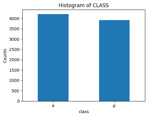
▶ The distribution of our target variable looks balanced.
Write a function for distributions
Since all data types are the same, that is object, we can write a function to use for all of them. We can do this with an iterative code that will give us all columns’ histogram at once, but to investigate every variable separately and thoroughly, I will use a function that will take a single column name as an argument instead.
# Define a function that will print a given column as histogram
# and the distribution of each value within by the target variable
# and their valuecounts

def countplot_vcounts(df, column_name):
  """Plots a histogram for a given column in a Pandas DataFrame and prints value counts.
  Args:
    df: The Pandas DataFrame.
    column_name: The name of the column to plot.
  """
  try:
    # Plotting the histogram
    plt.figure(figsize=(5, 4))
    sns.countplot(data=df, x=column_name, hue='class')
    plt.title(f'Countplot of {column_name.upper()} by Class')
    plt.xlabel(column_name)
    plt.ylabel('Count')
    plt.tight_layout()
    plt.show()

    # Printing value counts
    print(f"\nValue counts for {column_name.upper()}:\n")
    counts = df[column_name].value_counts()
    percs = df[column_name].value_counts(normalize=True).mul(100).round(1).astype(str) + '%'
    print(pd.concat([counts, percs], axis=1, keys=['count', 'percentage']))

  except KeyError:
    print(f"Error: Column '{column_name}' not found in the DataFrame.")
  except Exception as e:
    print(f"An unexpected error occurred: {e}")
3.2 Cap-Shape
# Plot Cap Shape vs Class
countplot_vcounts(df_study, 'cap-shape')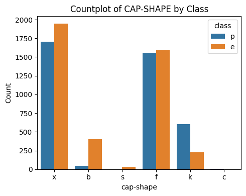
Value counts for CAP-SHAPE:

           count percentage
cap-shape
x           3656      45.0%
f           3152      38.8%
k            828      10.2%
b            452       5.6%
s             32       0.4%
c              4       0.0%
The values were:
- Cap Shape: bell=b, conical=c, convex=x, flat=f, knobbed=k, sunken=s
▶ Cap-Shape vs Class:
- The values ‘x‘ and ‘f‘ together holds ~84%.
- For ‘x‘ and ‘f‘ the Class distributions are quite balanced.
- Having a cap shape of ‘b‘ is more likely an indicator of the mushroom being ‘edible‘.
- Having a cap shape of ‘k‘ is more likely an indicator of the mushroom being ‘poisonous‘.
- The distributions of cap shape ‘s‘ and ‘c‘ are quite low.
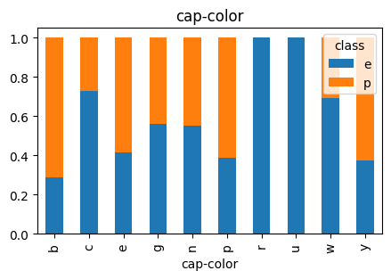
3.3 Cap-Color
# Plot Cap Color vs Class
countplot_vcounts(df_study, 'cap-color')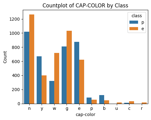
Value counts for CAP-COLOR:

           count percentage
cap-color
n           2284      28.1%
g           1840      22.6%
e           1500      18.5%
y           1072      13.2%
w           1040      12.8%
b            168       2.1%
p            144       1.8%
c             44       0.5%
u             16       0.2%
r             16       0.2%
The values were:
- Cap Color: brown=n, buff=b, cinnamon=c, gray=g, green=r, pink=p, purple=u, red=e, white=w, yellow=y
▶ Cap-Color vs Class:
- The values ‘n‘ and ‘g‘ together holds a little higher than half.
- For ‘n‘, ‘g‘ and ‘e‘ the Class distributions are close to being balanced, while ‘n’ and ‘g’ tend to have more ‘edible’, ‘e’ tend to have more ‘poisonuos’.
- Having a cap color of ‘w‘ is more likely an indicator of the mushroom being ‘edible‘.
- Having a cap color of ‘y‘ is more likely an indicator of the mushroom being ‘poisonous‘.
- The distributions of cap color ‘p‘ and ‘b‘ are low.
- The distributions of cap color ‘u‘, ‘c‘ and ‘r‘ are quite low.
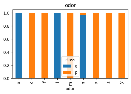
3.4 Odor
# Plot Odor vs Class
countplot_vcounts(df_study, 'odor')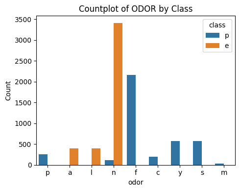
Value counts for ODOR:

      count percentage
odor
n      3528      43.4%
f      2160      26.6%
y       576       7.1%
s       576       7.1%
a       400       4.9%
l       400       4.9%
p       256       3.2%
c       192       2.4%
m        36       0.4%
The values were:
- Odor: almond=a, anise=l, creosote=c, fishy=y, foul=f, musty=m, none=n, pungent=p, spicy=s
▶ Odor vs Class:
- The values ‘n‘ and ‘f‘ together holds more than 70%.
- Having an odor of ‘n‘, ‘a‘ and ‘l‘ is more likely an indicator of the mushroom being ‘edible‘.
- Having an odor of ‘f‘, ‘y‘, ‘s‘, ‘p‘, ‘c‘ and ‘m‘ is more likely an indicator of the mushroom being ‘poisonous‘.
- Apart from ‘f‘ and ‘n‘, the distributions are low.
3.5 Habitat
# Plot Habitat vs Class
countplot_vcounts(df_study, 'habitat')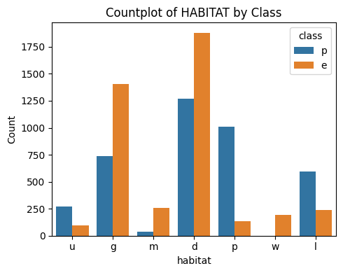
Value counts for HABITAT:

         count percentage
habitat
d         3148      38.7%
g         2148      26.4%
p         1144      14.1%
l          832      10.2%
u          368       4.5%
m          292       3.6%
w          192       2.4%
The values were:
- Habitat: grasses=g, leaves=l, meadows=m, paths=p, urban=u, waste=w, woods=d
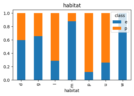
▶ Habitat vs Class:
- The values ‘d‘ and ‘g‘ together holds more than 65%.
- Having an habitat of ‘g‘, ‘d‘, ‘m‘ and ‘w‘ is more likely an indicator of the mushroom being ‘edible‘.
- Having an habitat of ‘p‘, ‘l‘ and’u‘ is more likely an indicator of the mushroom being ‘poisonous‘.
4 Machine Learning Models
The data will be split into train and test sets, then implied scaling and fit into seven different ML algorithms listed below. Finally the results will be compared.
- Logistic Regression
- Decision Tree
- Random Forest
- Gaussian Naive Bayes
- Support Vector Classification (SVC)
- K-Nearest Neighbors (KNN)
- XGBoost
# Import libraries for splitting, encoding, scaling and evaluation
from sklearn.model_selection import train_test_split
from sklearn.preprocessing import OneHotEncoder, StandardScaler, LabelEncoder
from sklearn.metrics import accuracy_score, classification_report, confusion_matrix

# Create a copy for models
df_model = df_study.copy()
# Separate Features and Target
X = df_model.drop("class", axis=1)
y = df_model["class"]
Since the target variable is binary, label encoding is used to convert ‘e’ and ‘p’ into 0 and 1.
# Encode the target variable to numeric values
label_encoder = LabelEncoder()
y_encoded = label_encoder.fit_transform(y)
# Train-test split
X_train, X_test, y_train, y_test = train_test_split(X, y_encoded, test_size=0.3, random_state=42)
Since there is no order between values, One-Hot encoding is used.
# Initialize OneHotEncoder
encoder = OneHotEncoder(drop="first", sparse_output=False)
    # drop first to avoid dummy variable trap

# Fit Encoder on Training Data and Transform Both Sets
X_train_encoded = encoder.fit_transform(X_train)  # Fit and transform on the training data
X_test_encoded = encoder.transform(X_test)        # Only transform on the test data
4.1 Logistic Regression
from sklearn.linear_model import LogisticRegressionLogistic regression (like many other linear models) performs best when features are on similar scales, especially when using gradient descent for optimization. Therefore I’ll perform Standardization with StandardScaler.
# Feature scaling: Standardize the features for Logistic Regression
scaler_lr = StandardScaler()
X_train_lr_scaled = scaler_lr.fit_transform(X_train_encoded)  # Fit and transform on training data
X_test_lr_scaled = scaler_lr.transform(X_test_encoded)        # Only transform on test data
# Train Logistic Regression Model
log_reg_model = LogisticRegression()
log_reg_model.fit(X_train_lr_scaled, y_train) # Fit the scaled data
# Make Predictions
y_pred_lr = log_reg_model.predict(X_test_lr_scaled)# Evaluate Model
print("Accuracy:", round(accuracy_score(y_test, y_pred_lr),3))
print("\nClassification Report:\n", classification_report(y_test, y_pred_lr, digits=3))Accuracy: 0.991
Classification Report:
precision recall f1-score support
0 0.984 1.000 0.992 1257
1 1.000 0.982 0.991 1181
accuracy 0.991 2438
macro avg 0.992 0.991 0.991 2438
weighted avg 0.992 0.991 0.991 2438
4.2 Decision Tree
from sklearn.tree import DecisionTreeClassifierDecision Tree do not require scaling, so I’ll use the encoded data directly.
# Use the encoded data directly
dt_model = DecisionTreeClassifier(random_state=42)
dt_model.fit(X_train_encoded, y_train)
y_pred_dt = dt_model.predict(X_test_encoded)

print("Accuracy:", round(accuracy_score(y_test, y_pred_dt), 3))
print("\nDecision Tree Classification Report:\n", classification_report(y_test, y_pred_dt, digits=3))
Accuracy: 0.997
Decision Tree Classification Report:
precision recall f1-score support
0 0.994 1.000 0.997 1257
1 1.000 0.994 0.997 1181
accuracy 0.997 2438
macro avg 0.997 0.997 0.997 2438
weighted avg 0.997 0.997 0.997 2438
4.3 Random Forest
from sklearn.ensemble import RandomForestClassifierNo scaling is required for Random Forest as well, so I’ll use the one-hot encoded data directly (X_train_encoded and X_test_encoded).
rf_model = RandomForestClassifier(random_state=42)
rf_model.fit(X_train_encoded, y_train)
y_pred_rf = rf_model.predict(X_test_encoded)

print("Accuracy:", round(accuracy_score(y_test, y_pred_rf),3))
print("\nRandom Forest Classification Report:\n", classification_report(y_test, y_pred_rf, digits=3))
Accuracy: 0.996
Random Forest Classification Report:
precision recall f1-score support
0 0.993 1.000 0.996 1257
1 1.000 0.992 0.996 1181
accuracy 0.996 2438
macro avg 0.996 0.996 0.996 2438
weighted avg 0.996 0.996 0.996 2438
4.4 Gaussian Naive Bayes
from sklearn.naive_bayes import GaussianNBNaive Bayes is a probabilistic classifier that assumes features follow a Gaussian (normal) distribution, which can work well for many classification tasks.
GNB doesn’t require scaling because it assumes that features follow a normal distribution. However, it is generally a good practice to use scaled data when dealing with Gaussian Naive Bayes, especially if features have different ranges or units.
gnb_model = GaussianNB()
gnb_model.fit(X_train_lr_scaled, y_train)  # Use scaled features for GNB
y_pred_gnb = gnb_model.predict(X_test_lr_scaled)

print("Accuracy:", round(accuracy_score(y_test, y_pred_gnb), 3))
print("\nGaussian Naive Bayes Classification Report:\n", classification_report(y_test, y_pred_gnb, digits=3))
Accuracy: 0.984
Gaussian Naive Bayes Classification Report:
precision recall f1-score support
0 0.971 1.000 0.985 1257
1 1.000 0.968 0.984 1181
accuracy 0.984 2438
macro avg 0.985 0.984 0.984 2438
weighted avg 0.985 0.984 0.984 2438
4.5 Support Vector Classification
from sklearn.svm import SVCSVM models are sensitive to the scale of the data. Therefore, it’s crucial to scale the features before applying SVC.
svc_model = SVC(random_state=42)
svc_model.fit(X_train_lr_scaled, y_train)         # Train on scaled data
y_pred_svc = svc_model.predict(X_test_lr_scaled)  # Predict on scaled data

print("Accuracy:", round(accuracy_score(y_test, y_pred_svc), 3))
print("\nSupport Vector Classification Report:\n", classification_report(y_test, y_pred_svc, digits=3))
Accuracy: 0.995
Support Vector Classification Report:
precision recall f1-score support
0 0.991 1.000 0.995 1257
1 1.000 0.990 0.995 1181
accuracy 0.995 2438
macro avg 0.995 0.995 0.995 2438
weighted avg 0.995 0.995 0.995 2438
4.6 K-Nearest Neighbors
from sklearn.neighbors import KNeighborsClassifierIt’s important to scale the features before applying KNN, as it relies on distance calculations between data points (typically Euclidean distance).
knn_model = KNeighborsClassifier(n_neighbors=3)   # Choose k=3 for this example
knn_model.fit(X_train_lr_scaled, y_train)         # Train on scaled data
y_pred_knn = knn_model.predict(X_test_lr_scaled)  # Predict on scaled data

print("Accuracy:", round(accuracy_score(y_test, y_pred_knn), 3))
print("\nSupport Vector Classification Report:\n", classification_report(y_test, y_pred_knn, digits=3))
Accuracy: 0.996
Support Vector Classification Report:
precision recall f1-score support
0 0.992 1.000 0.996 1257
1 1.000 0.992 0.996 1181
accuracy 0.996 2438
macro avg 0.996 0.996 0.996 2438
weighted avg 0.996 0.996 0.996 2438
4.7 XGBoost
import xgboost as xgbXGBoost (Extreme Gradient Boosting) is an efficient and powerful implementation of gradient boosting algorithms, and it’s widely used for classification tasks due to its high performance and flexibility.
xgb_model = xgb.XGBClassifier(random_state=42)
xgb_model.fit(X_train_lr_scaled, y_train)         # Train on scaled data
y_pred_xgb = xgb_model.predict(X_test_lr_scaled)  # Predict on scaled data

print("Accuracy:", round(accuracy_score(y_test, y_pred_xgb), 3))
print("\nXGBoost Classification Report:\n", classification_report(y_test, y_pred_xgb, digits=3))
Accuracy: 0.997
XGBoost Classification Report:
precision recall f1-score support
0 0.994 1.000 0.997 1257
1 1.000 0.993 0.997 1181
accuracy 0.997 2438
macro avg 0.997 0.997 0.997 2438
weighted avg 0.997 0.997 0.997 2438
5 Compare the Classification Algorithms
To summarize the above results the accuracy scores of all models are listed below.
Logistic Regression 0.991
Decision Tree 0.997
Random Forest 0.996
Gaussian Naive Bayes 0.984
Support Vector Classification 0.995
K-Nearest Neighbors 0.996
XGBoost 0.997
Models’ accuracy scores are almost perfect and very close to each other, only GNB has a slightly less score than others. However, as demonstrated above, all models’ f-1 score is the same as their accuracy score. This needs to be checked further.
Also, since we are trying to predict the poisonous mushrooms, the recall score (true positive rate) is a much more important metric than accuracy. For these reasons, the confusion matrix for all models is printed below.
5.1 Confusion Matrices for all models
from sklearn.metrics import confusion_matrix

# List of models and their names
models = [
    ("Logistic Regression", log_reg_model, X_train_lr_scaled, X_test_lr_scaled),
    ("Decision Tree", dt_model, X_train_encoded, X_test_encoded),
    ("Random Forest", rf_model, X_train_encoded, X_test_encoded),
    ("Gaussian Naive Bayes", gnb_model, X_train_lr_scaled, X_test_lr_scaled),
    ("Support Vector Classifier", svc_model, X_train_lr_scaled, X_test_lr_scaled),
    ("K-Nearest Neighbors", knn_model, X_train_lr_scaled, X_test_lr_scaled),
    ("XGBoost", xgb_model, X_train_lr_scaled, X_test_lr_scaled)
]

# Loop through models and print confusion matrices
for model_name, model, X_train_data, X_test_data in models:
    # Generate predictions
    y_pred = model.predict(X_test_data)

    # Compute confusion matrix
    conf_matrix = confusion_matrix(y_test, y_pred)

    # Print the confusion matrix
    print(f"Confusion Matrix for {model_name}:\n{conf_matrix}\n")
Confusion Matrix for Logistic Regression:
[[1257 0]
[ 21 1160]]
Confusion Matrix for Decision Tree:
[[1257 0]
[ 7 1174]]
Confusion Matrix for Random Forest:
[[1257 0]
[ 9 1172]]
Confusion Matrix for Gaussian Naive Bayes:
[[1257 0]
[ 38 1143]]
Confusion Matrix for Support Vector Classifier:
[[1257 0]
[ 12 1169]]
Confusion Matrix for K-Nearest Neighbors:
[[1257 0]
[ 10 1171]]
Confusion Matrix for XGBoost:
[[1257 0]
[ 8 1173]]
▶ All models predict the ‘edible’ mushrooms perfectly, they differ on predicting the ‘poisonous’ mushrooms that are much more important. While tree-based models (Decision Tree, Random Forest and XGB) perform best on predicting the ‘poisonous’ outcomes, GNB and Logistic Regression performed the worst. K-Nearest and SVC performed close to the tree-based models.
All models’ perfect performance on predicting ‘edible’ mushrooms could be a sign of a feature dominance and one of the main reasons for this could be the distribution within the ‘odor’ column as mentioned in EDA. All values within this column seem to be a significant factor toward predicting the mushrooms. Below code outputs the crosstab within this column.
5.2 Values in Odor column
for col in X.columns:
    pd.crosstab(X[col], y).div(pd.crosstab(X[col], y).sum(axis=1), axis=0).plot(
        kind='bar', stacked=True, figsize=(5, 3), title=col
    )
    plt.show()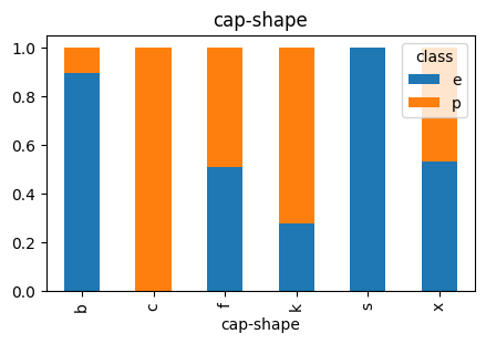
Unlike with other features, almost all values of Odor correspond uniquely to one outcome in the target variable (class), that’s why models strongly associate this column with that class. The only value in this column that holds both outcomes, ‘edible’ and ‘poisonous’, is ‘n’ and its distribution is heavily skewed towards ‘edible’. This might be the explanation for all models’ perfect prediction on ‘edible’ mushrooms.
5.3 The effect of a significant feature
To check the effect of ‘Odor’ on predictions, another round of ML training is performed, this time without the ‘Odor’ column as one of the features. The aim with this is to get another insight on models’ performances and characteristics.
For the simplicity of this report, the codes are not provided but the exact same steps were followed as demonstrated before, only without the column ‘Odor’. With the absence of this feature, the confusion matrix of all models reflects the below digits.
5.3.1 Confusion Matrices without ‘Odor’ for all models
# List of models and their names
models = [
    ("Logistic Regression", log_reg_model, X_train_lr_scaled, X_test_lr_scaled),
    ("Decision Tree", dt_model, X_train_encoded, X_test_encoded),
    ("Random Forest", rf_model, X_train_encoded, X_test_encoded),
    ("Gaussian Naive Bayes", gnb_model, X_train_lr_scaled, X_test_lr_scaled),
    ("Support Vector Classifier", svc_model, X_train_lr_scaled, X_test_lr_scaled),
    ("K-Nearest Neighbors", knn_model, X_train_lr_scaled, X_test_lr_scaled),
    ("XGBoost", xgb_model, X_train_lr_scaled, X_test_lr_scaled)
]
# Set up the figure with a grid layout for the subplots
fig, axes = plt.subplots(nrows=2, ncols=4, figsize=(14, 7))
axes = axes.ravel() # Flatten the 2D array of axes for easy indexing
# Loop through each model and plot the confusion matrix
for i, (model_name, model, X_train_data, X_test_data) in enumerate(models):
# Get the predictions for the current model
y_pred = model.predict(X_test_data)
# Calculate the confusion matrix
conf_matrix = confusion_matrix(y_test, y_pred)
# Plot the confusion matrix using seaborn heatmap
sns.heatmap(conf_matrix, annot=True, fmt="d", cmap="Blues",
xticklabels=["Edible (0)", "Poisonous (1)"],
yticklabels=["Edible (0)", "Poisonous (1)"], ax=axes[i])
# Set the title of the subplot
axes[i].set_title(f"{model_name} Conf. Matrix")
axes[i].set_ylabel("True Labels")
axes[i].set_xlabel("Predicted Labels")
# Adjust layout for better spacing
plt.tight_layout()
plt.show()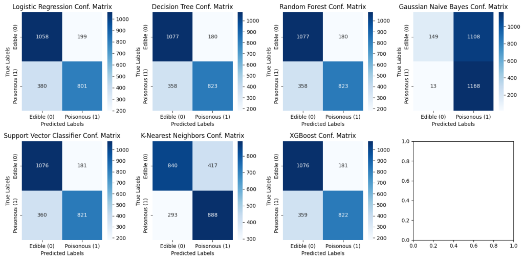
Removing out the column ‘Odor’ dramatically changes the predictions. To read the results better, let’s compare the models based on their True Positive and True Negative rates.
5.3.2 Predicting poisonous (True Positive Rate, or recall)
from sklearn.metrics import recall_score# Recall for all models
recall_scores = {
"Logistic Regression": recall_score(y_test, y_pred_lr, pos_label=1),
"Decision Tree": recall_score(y_test, y_pred_dt, pos_label=1),
"Random Forest": recall_score(y_test, y_pred_rf, pos_label=1),
"Gaussian Naive Bayes": recall_score(y_test, y_pred_gnb, pos_label=1),
"Support Vector Classifier": recall_score(y_test, y_pred_svc, pos_label=1),
"K-Nearest Neighbors": recall_score(y_test, y_pred_knn, pos_label=1),
"XGBoost": recall_score(y_test, y_pred_xgb, pos_label=1),
}# Plot the Recall scores with percentages
plt.figure(figsize=(8, 5))
bars = plt.bar(recall_scores.keys(), recall_scores.values(), color='orange', edgecolor='black')
# Add percentages to each bar
for bar in bars:
height = bar.get_height()
plt.text(
bar.get_x() + bar.get_width() / 2, # X-coordinate
height - 0.06, # Y-coordinate
f"{height * 100:.1f}%", # Format as percentage
ha='center', # Horizontal alignment
va='bottom', # Vertical alignment
fontsize=10, # Font size
color='black' # Text color
)
# Labels and styling
plt.xlabel('Models')
plt.ylabel('Recall (Positive Class)')
plt.title('Comparison of Recall Across Models')
plt.xticks(rotation=45, ha='right')
plt.ylim(0, 1) # Recall values range from 0 to 1
plt.tight_layout()
plt.show()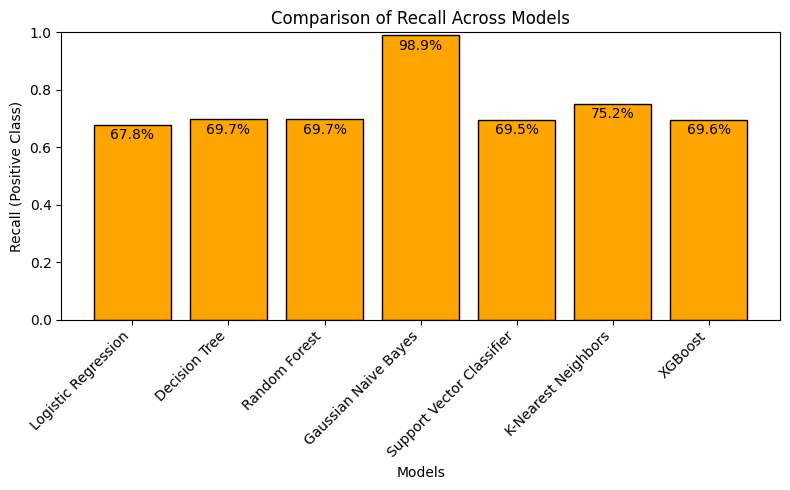
▶ Without the column ‘Odor’, tree-based models (Decision Tree, Random Forest, XGB), SVC and Logistic Regression (LR) perform similarly on predicting the ‘poisonous’ outcomes with around 70% recall, while LR has a slightly lower rate (~68%). K-Nearest Neighbors performs a little better than these models (~75%), and GNB performs almost perfectly with around 99% rate.
As seen in the above confusion matrix results, checking only the recall score does not give the full picture. K-NN and GNB’s better performances on recall is not repeating on their true negative rates.
5.3.3 Predicting edible (True Negative Rate)
# Confusion matrices for all models
conf_matrix_lr = confusion_matrix(y_test, y_pred_lr)    # Logistic Regression
conf_matrix_dt = confusion_matrix(y_test, y_pred_dt)    # Decision Tree
conf_matrix_rf = confusion_matrix(y_test, y_pred_rf)    # Random Forest
conf_matrix_nb = confusion_matrix(y_test, y_pred_gnb)   # Gaussian Naive Bayes
conf_matrix_svc = confusion_matrix(y_test, y_pred_svc)  # Support Vector Classifier
conf_matrix_knn = confusion_matrix(y_test, y_pred_knn)  # K-Nearest Neighbors
conf_matrix_xgb = confusion_matrix(y_test, y_pred_xgb)  # XGBoost
# Function to calculate TNR from a confusion matrix
def calculate_tnr(conf_matrix):
tn, fp, fn, tp = conf_matrix.ravel()
return tn / (tn + fp)
tnr_scores = {
"Logistic Regression": calculate_tnr(conf_matrix_lr),
"Decision Tree": calculate_tnr(conf_matrix_dt),
"Random Forest": calculate_tnr(conf_matrix_rf),
"Gaussian Naive Bayes": calculate_tnr(conf_matrix_nb),
"Support Vector Classifier": calculate_tnr(conf_matrix_svc),
"K-Nearest Neighbors": calculate_tnr(conf_matrix_knn),
"XGBoost": calculate_tnr(conf_matrix_xgb),
}# Plot the TNR scores with percentages
plt.figure(figsize=(8, 5))
bars = plt.bar(tnr_scores.keys(), tnr_scores.values(), color='skyblue', edgecolor='black')
# Add percentages to each bar
for bar in bars:
height = bar.get_height()
plt.text(
bar.get_x() + bar.get_width() / 2, # X-coordinate
height, # Y-coordinate
f"{height * 100:.1f}%", # Format as percentage
ha='center', # Horizontal alignment
va='bottom', # Vertical alignment
fontsize=10, # Font size
color='black' # Text color
)
# Labels and styling
plt.xlabel('Models')
plt.ylabel('True Negative Rate (TNR)')
plt.title('Comparison of True Negative Rates Across Models')
plt.xticks(rotation=45, ha='right')
plt.ylim(0, 1) # TNR values range from 0 to 1
plt.tight_layout()
plt.show()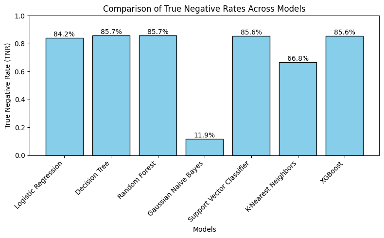
▶ Tree-based models (Decision Tree, Random Forest, XGB), SVC and Logistic Regression (LR) perform similarly on predicting the ‘edible’ outcomes with around 86% TNR, while LR has a slightly lower rate (~84%). K-Nearest Neighbors performs much worse than these models (~67%), and GNB performs extremely low with around only 12% rate.
5.4 Concluding Remarks
As demonstrated above, specific features can affect a model’s performance tremendously. Here domain knowledge plays a crucial role when it comes to considering a dominant feature (such as Odor) to fit in the model or not. Also, this study points out two more questions:
Why do GNB and KNN behave differently?
GNB assumes that features are independent (a strong assumption called the “Naive” assumption) and features follow a Gaussian distribution for each class. Without Odor, the Gaussian assumption becomes more critical. If the remaining features (cap-shape, cap-color, etc.) are non-Gaussian or poorly independent, GNB struggles to form reliable decision boundaries.
The drastic drop in TNR (~12%) suggests that GNB is over-predicting the positive class (poisonous mushrooms). The model likely assigns high probabilities to the positive class due to misinterpretation of the remaining features.
KNN relies on proximity in the feature space, though it can be sensitive to irrelevant or noisy features, explaining its drop to ~67% TNR.
Why Do Other Models Maintain Higher TNR Without Odor?
Other models (e.g., Decision Tree, Random Forest, Logistic Regression, etc.) are more robust to violations of independence and Gaussian assumptions. Tree-based models can handle nonlinear interactions and categorical splits effectively. SVM and Logistic Regression perform well if the data is reasonably separable, even without Odor.
The consistent drop in TNR across most models (to ~85%) after removing Odor suggests that this feature was a major driver of separability between classes. In fact, similar studies revealed that the importance score of the Odor variable was extremely high (Ortiz-Letechipia et al. 2024)*.
6 Going Forward
Takeaways
What I learned:
The behavior we observed highlights the importance of understanding how different models interact with specific features. GNB’s drastic performance shift is a great example of how strong model assumptions can lead to overfitting or poor generalization. While GNB might not be the best choice for this dataset without Odor, the robustness of other models makes them better candidates for real-world scenarios.
However, there might be situations where the recall scores are extremely important so we would effort some compensation on true negative scores. In such cases GNB could be our champion model.
Next Steps
For next steps, further studies could be performed focusing on tree-based models and with different arguments within each of the algorithms.
* Alternative link to the research paper: “Classification and selection of the main features for the identification of toxicity in Agaricus and Lepiota with machine learning algorithms”.
Previous Data Project

Next Data Project

Browse my projects by category:
ALL • Data • UX • Arch