Review
This notebook is a continuation of the bank churn project. Below is a recap of the considerations and decisions that we’ve already made.
- Modeling objective: To predict whether a customer will churn, a binary classification task.
- Target variable:
Exitedcolumn, 0 or 1. - Class balance: The data is imbalanced 80/20 (not churned/churned), but we will not perform class balancing.
- Primary evaluation metric: F1 score.
- Modeling workflow and model selection: The champion model will be the model with the best validation F1 score. Only the champion model will be used to predict on the test data.
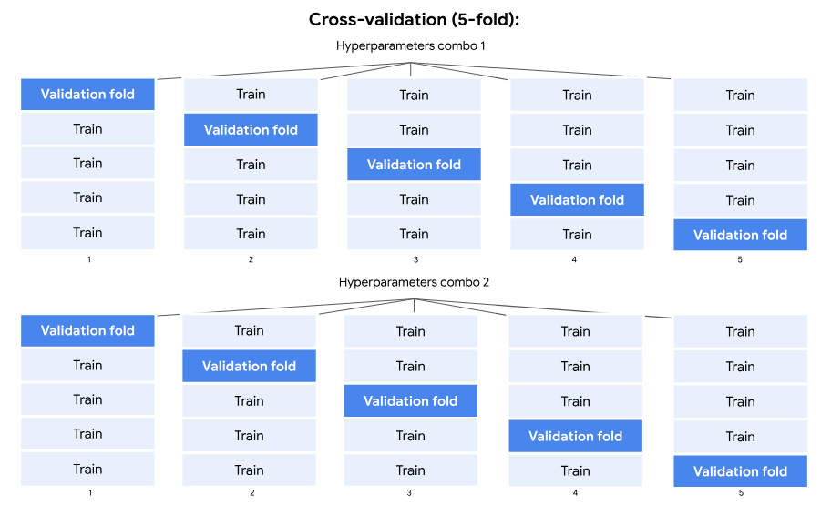
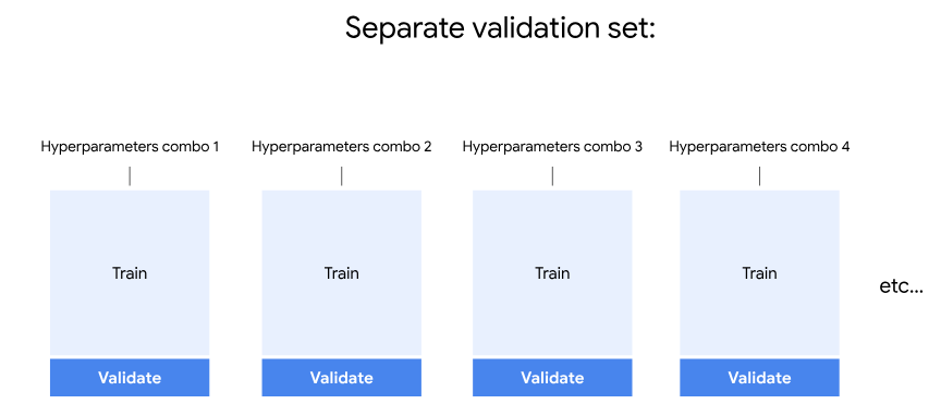
A note on cross-validation/validation
This notebook is for teaching purposes. As such, it includes two approaches to validation: cross-validating the training data and validating using a separate validation dataset. In practice, we generally will only use one or the other for a given project.
Cross-validation is more rigorous, because it maximizes the usage of the training data, but if we have a very large dataset or limited computing resources, it may be better to validate with a separate validation dataset.
Import and Read
import numpy as np
import pandas as pd

import matplotlib.pyplot as plt

# This lets us see all of the columns, preventing Jupyter from redacting them
pd.set_option('display.max_columns', None)

from sklearn.model_selection import GridSearchCV, train_test_split
from sklearn.metrics import accuracy_score, precision_score, recall_score,\
f1_score, confusion_matrix, ConfusionMatrixDisplay

from sklearn.ensemble import RandomForestClassifier

# This module lets us save our models once we fit them
import pickle
# Read in data
file = 'Churn_Modelling.csv'
df_original = pd.read_csv(file)
df_original.head()| RowNumber | CustomerId | Surname | CreditScore | Geography | Gender | Age | Tenure | Balance | NumOfProducts | HasCrCard | IsActiveMember | EstimatedSalary | Exited | |
|---|---|---|---|---|---|---|---|---|---|---|---|---|---|---|
| 0 | 1 | 15634602 | Hargrave | 619 | France | Female | 42 | 2 | 0.00 | 1 | 1 | 1 | 101348.88 | 1 |
| 1 | 2 | 15647311 | Hill | 608 | Spain | Female | 41 | 1 | 83807.86 | 1 | 0 | 1 | 112542.58 | 0 |
| 2 | 3 | 15619304 | Onio | 502 | France | Female | 42 | 8 | 159660.80 | 3 | 1 | 0 | 113931.57 | 1 |
| 3 | 4 | 15701354 | Boni | 699 | France | Female | 39 | 1 | 0.00 | 2 | 0 | 0 | 93826.63 | 0 |
| 4 | 5 | 15737888 | Mitchell | 850 | Spain | Female | 43 | 2 | 125510.82 | 1 | 1 | 1 | 79084.10 | 0 |
Feature engineering
Feature selection
# Drop useless and sensitive (Gender) cols
churn_df = df_original.drop(['RowNumber', 'CustomerId', 'Surname', 'Gender'], axis=1)
churn_df.head()| CreditScore | Geography | Age | Tenure | Balance | NumOfProducts | HasCrCard | IsActiveMember | EstimatedSalary | Exited | |
|---|---|---|---|---|---|---|---|---|---|---|
| 0 | 619 | France | 42 | 2 | 0.00 | 1 | 1 | 1 | 101348.88 | 1 |
| 1 | 608 | Spain | 41 | 1 | 83807.86 | 1 | 0 | 1 | 112542.58 | 0 |
| 2 | 502 | France | 42 | 8 | 159660.80 | 3 | 1 | 0 | 113931.57 | 1 |
| 3 | 699 | France | 39 | 1 | 0.00 | 2 | 0 | 0 | 93826.63 | 0 |
| 4 | 850 | Spain | 43 | 2 | 125510.82 | 1 | 1 | 1 | 79084.10 | 0 |
Feature transformation
# Dummy encode categoricals
churn_df2 = pd.get_dummies(churn_df, drop_first='True')
churn_df2.head()| CreditScore | Age | Tenure | Balance | NumOfProducts | HasCrCard | IsActiveMember | EstimatedSalary | Exited | Geography_Germany | Geography_Spain | |
|---|---|---|---|---|---|---|---|---|---|---|---|
| 0 | 619 | 42 | 2 | 0.00 | 1 | 1 | 1 | 101348.88 | 1 | 0 | 0 |
| 1 | 608 | 41 | 1 | 83807.86 | 1 | 0 | 1 | 112542.58 | 0 | 0 | 1 |
| 2 | 502 | 42 | 8 | 159660.80 | 3 | 1 | 0 | 113931.57 | 1 | 0 | 0 |
| 3 | 699 | 39 | 1 | 0.00 | 2 | 0 | 0 | 93826.63 | 0 | 0 | 0 |
| 4 | 850 | 43 | 2 | 125510.82 | 1 | 1 | 1 | 79084.10 | 0 | 0 | 1 |
Split the data
# Define the y (target) variable
y = churn_df2["Exited"]

# Define the X (predictor) variables
X = churn_df2.copy()
X = X.drop("Exited", axis = 1)

# Split into train and test sets
X_train, X_test, y_train, y_test = train_test_split(X, y, test_size=0.25, stratify=y, random_state=42)
Modeling
Cross-validated hyperparameter tuning
The cross-validation process is the same as it was for the decision tree model. The only difference is that we’re tuning more hyperparameters now. The steps are included below as a review.
For details on cross-validating with GridSearchCV, refer back to the GridSearchCV documentation in scikit-learn.
- Instantiate the classifier (and set the
random_state). - Create a dictionary of hyperparameters to search over.
- Create a set of scoring metrics to capture.
- Instantiate the
GridSearchCVobject. Pass as arguments:- The classifier (
rf) - The dictionary of hyperparameters to search over (
cv_params) - The set of scoring metrics (
scoring) - The number of cross-validation folds you want (
cv=5) - The scoring metric that we want GridSearch to use when it selects the “best” model (i.e., the model that performs best on average over all validation folds) (
refit='f1')
- The classifier (
- Fit the data (
X_train,y_train) to theGridSearchCVobject (rf_cv).
Note that we use the %%time magic at the top of the cell. This outputs the final runtime of the cell. (Magic commands, often just called “magics,” are commands that are built into IPython to simplify common tasks. They begin with % or %%.)
%%time

rf = RandomForestClassifier(random_state=0)

cv_params = {'max_depth': [2,3,4,5, None],
             'min_samples_leaf': [1,2,3],
             'min_samples_split': [2,3,4],
             'max_features': [2,3,4],
             'n_estimators': [75, 100, 125, 150]
             }

scoring = {'accuracy', 'precision', 'recall', 'f1'}

rf_cv = GridSearchCV(rf, cv_params, scoring=scoring, cv=5, refit='f1')

# rf_cv.fit(X_train, y_train)
CPU times: user 44 µs, sys: 22 µs, total: 66 µs
Wall time: 70.3 µs
Random forest validation on separate dataset
Now we’ll focus on:
- Using
pickleto save a fit model - Using a separate dataset to tune hyperparameters and validate our model
- Splitting the training data to create a validation dataset
- Creating a list of split indices to use with
PredefinedSplitsoGridSearchCVperforms validation on this defined validation set
Pickle
When models take a long time to fit, we don’t want to have to fit them more than once. If our kernel disconnects or we shut down the notebook and lose the cell’s output, we’ll have to refit the model, which can be frustrating and time-consuming.
pickle is a tool that saves the fit model object to a specified location, then quickly reads it back in. It also allows us to use models that were fit somewhere else, without having to train them ourselves.
# Define a path to the folder where you want to save the model
path = '/home/jovyan/work/'
This step will Write (i.e., save) the model, in Binary (hence, wb), to the folder designated by the above path. In this case, the name of the file we’re writing is rf_cv_model.pickle.
# Pickle the model
with open(path+'rf_cv_model.pickle', 'wb') as to_write:
    pickle.dump(rf_cv, to_write)
Once we save the model, we’ll never have to re-fit it when we run this notebook. Ideally, we could open the (Jupyter) notebook, select “Run all,” and the cells would run successfully all the way to the end without any model retraining.
For this to happen, we’ll need to return to the cell where we defined our grid search and comment out the line where we fit the model. Otherwise, when we re-run the notebook, it would refit the model.
Similarly, we’ll also need to go back to where we saved the model as a pickle and comment out those lines.
Next, we’ll add a new cell that reads in the saved model from the folder we already specified. For this, we’ll use rb (read binary) and be sure to assign the model to the same variable name as we used above, rf_cv.
# Read in pickled model
with open(path + 'rf_cv_model.pickle', 'rb') as to_read:
    rf_cv = pickle.load(to_read)
Now everything above is ready to run quickly and without refitting. We can continue by using the model’s best_params_ attribute to check the hyperparameters that had the best average F1 score across all the cross-validation folds.
rf_cv.fit(X_train, y_train)
rf_cv.best_params_
{'max_depth': None,
'max_features': 4,
'min_samples_leaf': 2,
'min_samples_split': 2,
'n_estimators': 125}
And to check the best average F1 score of this model on the validation folds, we can use the best_score_ attribute. Remember, if we had instead set refit=recall when we instantiated our GridSearchCV object earlier, then calling best_score_ would return the best recall score, and the best parameters might not be the same as what they are in the above cell, because the model would be optimizing for a different metric.
rf_cv.best_score_0.580528563620339
Our model had an F1 score of 0.5805, not terrible. Recall that when we ran our grid search, we specified that we also wanted to capture precision, recall, and accuracy. The reason for doing this is that it’s difficult to interpret an F1 score. These other metrics are much more directly interpretable, so they’re worth knowing.
The following cell defines a helper function that extracts these scores from the fit GridSearchCV object and returns a pandas dataframe with all four scores from the model with the best average F1 score during validation.
def make_results(model_name, model_object):
    '''
    Accepts as arguments a model name (your choice - string) and
    a fit GridSearchCV model object.
    Returns a pandas df with the F1, recall, precision, and accuracy scores
    for the model with the best mean F1 score across all validation folds.
    '''
    # Get all the results from the CV and put them in a df
    cv_results = pd.DataFrame(model_object.cv_results_)

    # Isolate the row of the df with the max(mean f1 score)
    best_estimator_results = cv_results.iloc[cv_results['mean_test_f1'].idxmax(), :]

    # Extract accuracy, precision, recall, and f1 score from that row
    f1 = best_estimator_results.mean_test_f1
    recall = best_estimator_results.mean_test_recall
    precision = best_estimator_results.mean_test_precision
    accuracy = best_estimator_results.mean_test_accuracy

    # Create table of results
    table = pd.DataFrame({'Model': [model_name],
                          'F1': [f1],
                          'Recall': [recall],
                          'Precision': [precision],
                          'Accuracy': [accuracy]
                         }
                        )

    return table
# Make a results table for the rf_cv model using above function
rf_cv_results = make_results('Random Forest CV', rf_cv)
rf_cv_results| Model | F1 | Recall | Precision | Accuracy | |
|---|---|---|---|---|---|
| 0 | Random Forest CV | 0.580529 | 0.472517 | 0.756289 | 0.861333 |
We can concatenate these results to our master results table from when we built the single decision tree model.
# Read in master results table
results = pd.read_csv('results1.csv', index_col=0)
results| Model | F1 | Recall | Precision | Accuracy | |
|---|---|---|---|---|---|
| 0 | Tuned Decision Tree | 0.560655 | 0.469255 | 0.701608 | 0.8504 |
# Concatenate the random forest results to the master table
results = pd.concat([rf_cv_results, results])
results
| Model | F1 | Recall | Precision | Accuracy | |
|---|---|---|---|---|---|
| 0 | Random Forest CV | 0.580529 | 0.472517 | 0.756289 | 0.861333 |
| 0 | Tuned Decision Tree | 0.560655 | 0.469255 | 0.701608 | 0.850400 |
The scores in the above table tell us that the random forest model performs better than the single decision tree model on every metric.
Now, let’s build another random forest model, only this time we’ll tune the hyperparameters using a separate validation dataset.
Modeling
Hyperparameters tuned with separate validation set
Begin by splitting the training data to create a validation dataset. Remember, we won’t touch the test data at all. We’ll use train_test_split to divide X_train and y_train into 80% training data (X_tr, y_tr) and 20% validation data (X_val, y_val).
# Create separate validation data
X_tr, X_val, y_tr, y_val = train_test_split(X_train, y_train, test_size=0.2,
                                            stratify=y_train, random_state=10)
When we tune hyperparameters with GridSearchCV using a separate validation dataset, we have to take a few extra steps. GridSearchCV wants to cross-validate the data. In fact, if the cv argument were left blank, it would split the data into five folds for cross-validation by default.
We don’t want it to do this. Instead, we’re going to tell it exactly which rows of X_train are for training, and which rows are for validation.
To do this, we need to make a list of length len(X_train) where each element is either a 0 or -1. A 0 in index i will indicate to GridSearchCV that index i of X_train is to be held out for validation. A -1 at a given index will indicate that that index of X_train is to be used as training data.
We’ll make this list using a list comprehension that looks at the index number of each row in X_train. If that index number is in X_val‘s list of index numbers, then the list comprehension appends a 0. If it’s not, then it appends a -1.
So if our training data is:
[A, B, C, D],
and our list is:
[-1, 0, 0, -1],
then GridSearchCV will use a training set of [A, D] and validation set of [B, C].
# Create list of split indices
split_index = [0 if x in X_val.index else -1 for x in X_train.index]
Now that we have this list, we need to import a new function called PredefinedSplit. This function is what allows us to pass the list we just made to GridSearchCV. (More about this function is in the documentation.)
from sklearn.model_selection import PredefinedSplitNow we can build the model. Everything is the same as when we cross-validated, except this time we pass the split_index list to the PredefinedSplit function and assign it to a new variable called custom_split. Then we’ll use this variable for the cv argument when we instantiate GridSearchCV.
rf = RandomForestClassifier(random_state=0)

cv_params = {'max_depth': [2,3,4,5, None],
             'min_samples_leaf': [1,2,3],
             'min_samples_split': [2,3,4],
             'max_features': [2,3,4],
             'n_estimators': [75, 100, 125, 150]
             }

scoring = {'accuracy', 'precision', 'recall', 'f1'}

custom_split = PredefinedSplit(split_index)

rf_val = GridSearchCV(rf, cv_params, scoring=scoring, cv=custom_split, refit='f1')
Now let’s fit the model.
rf_val.fit(X_train, y_train)CPU times: user 3min 51s, sys: 1.2 s, total: 3min 53s
Wall time: 3min 53s
GridSearchCV(cv=PredefinedSplit(test_fold=array([-1,  0, ..., -1, -1])),
             error_score=nan,
             estimator=RandomForestClassifier(bootstrap=True, ccp_alpha=0.0,
                                              class_weight=None,
                                              criterion='gini', max_depth=None,
                                              max_features='auto',
                                              max_leaf_nodes=None,
                                              max_samples=None,
                                              min_impurity_decrease=0.0,
                                              min_impurity_split=None,
                                              min_samples_leaf=1,
                                              min_samples_split=2,
                                              min_weigh...
                                              oob_score=False, random_state=0,
                                              verbose=0, warm_start=False),
             iid='deprecated', n_jobs=None,
             param_grid={'max_depth': [2, 3, 4, 5, None],
                         'max_features': [2, 3, 4],
                         'min_samples_leaf': [1, 2, 3],
                         'min_samples_split': [2, 3, 4],
                         'n_estimators': [75, 100, 125, 150]},
             pre_dispatch='2*n_jobs', refit='f1', return_train_score=False,
             scoring={'f1', 'recall', 'accuracy', 'precision'}, verbose=0)
Notice that this took less time than when we cross-validated, about 1/5 of the time. This is because during cross-validation the training data was divided into five folds. An ensemble of trees was grown with a particular combination of hyperparameters on four folds of data, and validated on the fifth fold that was held out. This whole process happened for each of five holdout folds. Then, another ensemble was trained with the next combination of hyperparameters, repeating the whole process. This continued until there were no more combinations of hyperparameters to run.
But now that we’re using a separate validation set, an ensemble is built for each combination of hyperparameters. Each ensemble is trained on the new training set and validated on the validation set. But this only happens one time for each combination of hyperparameters, instead of five times with cross-validation. That’s why the training time was only a fifth as long.
Let’s pickle the model.
# Pickle the model
with open(path+'rf_val_model.pickle', 'wb') as to_write:
    pickle.dump(rf_val, to_write)
We need to comment out where we fit the model and wrote the pickle, then read back in the pickled model.
# Open pickled model
with open(path+'rf_val_model.pickle', 'rb') as to_read:
    rf_val = pickle.load(to_read)
Now check the parameters of the best-performing model on the validation set:
rf_val.best_params_{'max_depth': None,
'max_features': 4,
'min_samples_leaf': 1,
'min_samples_split': 3,
'n_estimators': 150}
Notice that the best hyperparameters were slightly different than the cross-validated model.
Now, we’ll generate the model results using the make_results function, add them to the master table, and then sort them by F1 score in descending order.
# Create model results table
rf_val_results = make_results('Random Forest Validated', rf_val)

# Concatentate model results table with master results table
results = pd.concat([rf_val_results, results])

# Sort master results by F1 score in descending order
results.sort_values(by=['F1'], ascending=False)| Model | F1 | Recall | Precision | Accuracy | |
|---|---|---|---|---|---|
| 0 | Random Forest CV | 0.580529 | 0.472517 | 0.756289 | 0.861333 |
| 0 | Random Forest Validated | 0.575510 | 0.460784 | 0.766304 | 0.861333 |
| 0 | Tuned Decision Tree | 0.560655 | 0.469255 | 0.701608 | 0.850400 |
We can save the new master table to use later when we build more models.
# Save the master results table
results.to_csv(path+'results2.csv', index=False)
Model selection and final results
Now we have three models. If we’ve decided that we’re done trying to optimize them, then we can now use our best model to predict on the test holdout data. We’ll be using the cross-validated model without the depth limitation, but if we were instead to use the model that was validated against a separate validation dataset, we’d now go back and retrain the model on the full training set (training + validation sets).
Note: It might be tempting to see how all models perform on the test holdout data, and then to choose the one that performs best. While this can be done, it biases the final model, because we used our test data to go back and make an upstream decision. The test data should represent unseen data. In competitions, for example, we must submit our final model before receiving the test data.
The results in the table above tell us that the cross-validated random forest model performs a little better than the one trained on a separate validation set.
It performs well for precision and accuracy, but the recall is 0.4725. This means that out of all the people in the validation folds who actually left the bank, the model successfully identifies 47% of them.
We will not apply the model to the test data yet, because there is still one more model to build. Once we train that model, we’ll use our champion model to predict on the test data.
Disclaimer: Like most of my posts, this content is intended solely for educational purposes and was created primarily for my personal reference. At times, I may rephrase original texts, and in some cases, I include materials such as graphs, equations, and datasets directly from their original sources.
I typically reference a variety of sources and update my posts whenever new or related information becomes available. For this particular post, the primary source was Google Advanced Data Analytics Professional Certificate program.