Regression Analysis (or Regression Models) is a group of statistical techniques that use existing data to estimate the relationships between a single dependent variable and one or more independent variables.
PACE in Regression Analysis
In regression modeling, the Plan stage is about understanding our data in the problem context. Knowledge we bring, whether from industry or others, can be instrumental in the plan stage. We can do this by considering what data we have access to, how the data was collected, and what the business needs are.
In the Analyze stage, we examine our data more closely so we can choose a model or a couple of models we think might be appropriate.
Model assumptions are statements about the data that must be true to justify the use of particular data techniques. As a data professional, we will use statistics to check whether model assumptions are met.
For regression analysis, the Construct phase is where we actually build the model in Python (or other coding language of choice). This step involves selecting variables, transforming the data as needed, and writing code.
Even though we checked model assumptions before we built the model, many model assumptions need to be rechecked after the model is built.
The last part of the construct phase is evaluating the model results. At this point, we are answering the questions, how good is our model? We’ll choose metrics, compare models, and get preliminary results. Then based on our evaluation, we can use EDA to refine our model accordingly.
In the Execute phase we’ll interpret everything we learned from analyzing and constructing to share the story. We’ll prepare formal results and visualizations and share them with stakeholders.
To do this, we’ll convert model statistics into statements describing the relationship between the variables in the data. These descriptions must consider the context and initial questions from the plan phase.
However PACE is iterative, we might switch the order or repeat steps depending on the situation.
Linear Regression
The linear in linear regression indicates the relationship we can visualize on a graph, a line. A line is a collection of an infinite number of points extending in two opposite directions.
Linear regression is a technique that estimates the linear relationship between a continuous dependent variable y and one or more independent variables x.
Dependent variable (Y) is the variable a given model estimates, also referred to as a response or outcome variable. We assume that the dependent variable tends to vary based on the values of independent variables.
Independent variable (X) is a variable that explains trends in the dependent variable, also referred to as an explanatory or predictor variable.
Y = slope * X + intercept
The slope refers to the amount we expect y (the dependent variable) to increase or decrease per one unit increase of x (the independent variable). The intercept is the value of y when x equals 0.
When two variables, x and y, are related in a linear way, we say they are correlated. Using statistics, we can actually calculate how strong the linear relationship between x and y is.
There are two kinds of correlation, positive and negative: Positive correlation is a relationship between two variables that tend to increase or decrease together. Negative correlation, on the other hand, is an inverse relationship between two variables. When one variable increases, the other variable tends to decrease. The reverse is true too.
Determining linear relationships helps us answer questions such as,
- Which factors are associated with an increase or decrease in product sales?
- Which factors make social service providers increase resources in a given region?
- Which factors lead to more or less demand for public transportation?
However, it is important to note that correlation is not causation. When modeling variable relationships, a data scientist must be mindful of the extent of their claims.
Causation describes a cause and effect relationship where one variable directly causes the other to change in a particular way. Proving causation statistically requires much more rigorous methods and data collection than correlation. For a data professional, the distinction between correlation and causation is especially important when presenting results.
Articulating that correlation is not causation is part of a data professionals best practices and ethical toolbox. Both correlational and causal relationships provide useful insights. Regression analysis helps data analytics professionals tell nuanced stories without needing to prove causation.
Linear regression equation
The observed values or actual values, are the existing sample of data. Each data point in this sample is represented by an observed value of the dependent variable and an observed value of the independent variable.
Linear regression equation:
μ{Y|X} = β0 + β1X
In statistics, the intercept is written as Beta 0, which we sometimes call Beta naught, and the slope is written as Beta 1.
mu of y and the Betas are sometimes called parameters. Parameters are properties of populations and not samples. We can never know their true value since we can’t observe the whole population. But we can calculate estimates of the parameters using our sample data.
Linear regression estimation:
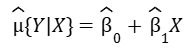
To differentiate between the population parameters and the estimates of the parameters, we denote the estimates with the hat. Beta 0 hat, Beta 1 hat, and mu hat, are all parameter estimates. Although it’s valuable to recognize the mu notation, we can use a simplified notation.
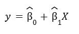
These estimated Betas are also called regression coefficients, represented as ![]() .
.
But how did we arrive at those regression coefficients?
One of the most common ways to calculate linear regression coefficients is ordinary least squares estimation, or OLS for short.
In linear regression analysis, we are trying to minimize something called a loss function. The loss function is a function that measures the distance between the observed values and the model’s estimated values.
Theoretically, we could draw an infinite number of lines that model the data we have. But we don’t want to find just any line. We want to find the best fit line. We want to minimize the loss function.
Logistic Regression
Logistic regression is a technique that models a categorical dependent variable based on one or more independent variables. The dependent variable can have two or more possible discrete values.
We use logistic regression to model complex probability problems. For example,
- What factors lead to someone subscribing or not subscribing to a newsletter?
- Under what circumstances does someone comment on an online video or social media post?
- Given certain factors, how likely is it that someone renews their membership to an organization?
Logistic regression equation
Logistic regression model:
μ{Y|X} = Prob(Y=1 | X)
The key concept is that the mean of y given x is equal to the probability of y equals one given x. Sometimes the probability of y given x is written as ‘p‘ to reinforce the idea of probability.
μ{Y|X} = Prob(Y=1 | X) = p
Now we want to understand what variables help explain those probabilities. Mathematically, we need a way to relate the x variables to the probability that y equals one.
β0 + β1X → ? → Prob(Y=1 | X)
In logistic regression, we use a link function to express the relationship between the x’s and the probability that y equals some outcome:
g(p) = β0 + β1X
A link function is a nonlinear function that connects or links the dependent variable to the independent variables mathematically.
A Quick Recap: Linear or Logistic
Similarities and differences between modeling approaches:
- Linear regression involves a y that is continuous, like book sales. While logistic regression involves a y that is categorical, like newsletter subscription.
- Since the linear regression model is a continuous variable, we’re estimating the mean of y. But logistic regression models a categorical variable, so we’re modeling the probability of an outcome.
- For linear regression, we can express y directly as a function of x. But for logistic regression, we need a link function to connect the probability of y with x.
| Linear Regression | Logistic Regression |
| Continuous data (i.e. book sales – 270 books, 754 books, etc.) | Categorical data (i.e. newsletter subscription – Yes / No) * |
| Estimating the MEAN of y | Estimating the PROBABILITY of an outcome |
| μ{Y|X} = β0 + β1X | μ{Y|X} = Prob(Y=1 | X) = p g(p) = β0 + β1X |
* This is a logistic regression with just two categories. But there are more complex versions of logistic regression that can model multiple outcomes or categories, such as types of skincare products people buy, or types of services that people receive.
Disclaimer: Like most of my posts, this content is intended solely for educational purposes and was created primarily for my personal reference. At times, I may rephrase original texts, and in some cases, I include materials such as graphs, equations, and datasets directly from their original sources.
I typically reference a variety of sources and update my posts whenever new or related information becomes available. For this particular post, the primary source was Google Advanced Data Analytics Professional Certificate.