Simple linear regression is a technique that estimates the linear relationship between one independent variable, X, and one continuous dependent variable, Y.
Ordinary least squares estimation
Equation for a regression line is:
y = intercept + slope * X
y = β0 + β1X
There are many different lines we could draw that might fit the data. However, we’re looking for the best fit line: The line that fits the data best by minimizing a loss function or error.
In order to find the best fit line, we need to measure error. We can consider error as some difference between the data we have, the observed values, and the predicted values generated by a given model.
The predicted values are the estimated y values for each x calculated by a model. The difference between observed or actual values and the predicted values of the regression line are what’s known as a residual.
The equation for residual value is:
Residual = observed value – predicted value
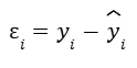
Epsilon resembles the letter E, as in E for error.
We can calculate individual residuals for each data point. An important thing to note is that the sum of the residuals is always equal to zero for OLS estimators. But for some estimators, the sum of the residuals is not always equal to zero.
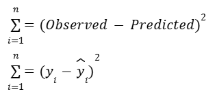
In order to capture a summary of total error in the model, we square each residual and then add up the residuals for every data point. This is called the sum of squared residuals.
The sum of squared residuals (SSR), is the sum of the squared differences between each observed value and the associated predicted value.
For linear regression, we’ll be using a technique called ordinary least squares to get our best-fit line.
Ordinary least squares (OLS) is a method that minimizes the sum of squared residuals to estimate parameters in a linear regression model.
Through trial and error, we can pick a line that we think is closest to the data points. But that’s very time-consuming. However in Python, the computer will use the ordinary least squares estimation technique to test out many lines and identify which one is the best fit line.
Estimating beta coefficients
We could keep adjusting the slope and intercept, and then calculating the predicted values, residuals, and squared residuals. But there’s really no way to be sure we’ve found the best fit line. Through advanced math, some formulas have been derived to find the beta coefficients that minimize error.
There are multiple ways to write out the formulas for finding the beta coefficients. For simple linear regression, one way to write the formulas is as follows:
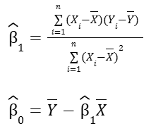
Now it may look confusing, but under my Math notes, I wrote about minimizing the squared error of the regression line and then examined the connection between the covariance and the regression line. Those posts try to explain how we get these formulas.
Correlation and the intuition behind simple linear regression
Correlation is a measurement of the way two variables move together. And remember a continuous variable can be summarized using some basic numbers. Two of these summary statistics are:
- Average: A measurement of central tendency (mean, median, or mode)
- Standard deviation: A measurement of spread
When two variables are summarized together, there is another relevant statistic called r, Pearson’s correlation coefficient, or simply the linear correlation coefficient. The correlation coefficient quantifies the strength of the linear relationship between two variables. It always falls in the range of [-1, 1].
- When r is negative, there is a negative correlation between the variables: as one increases, the other decreases.
- When r is positive, there is a positive correlation between the variables: as one increases, so too does the other.
- When r = 0, there is no linear correlation between the variables.
Note that there are cases where one variable might be precisely determined by another —like y=x2 or y=sin(x)— but the value of the linear correlation between X and Y would nonetheless be low or zero because their relationship is non-linear.
However, r only tells us the strength of the linear correlation between the variables; it does not tell us anything about the magnitude of the slope of the relationship between the variables aside from its sign.
The formula for r is:
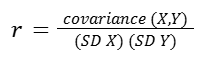
where:
Note: The formulas for r and covariance given here represent those used for entire populations. For samples, the denominator of the covariance formula is n – 1 and, similarly, the standard deviations in the formula for r are calculated using n – 1 instead of n.
Again, under my Math notes, there is a sample calculation of correlation coefficient, r. In another post, Variance and Standard Deviation of a Sample, I also examined why it’s better to use n-1, rather than n for samples.
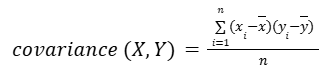
An easier way of thinking about this calculation is: the numerator (the covariance) represents the extent to which X and Y vary together from their respective means. When this value is positive, it suggests that high values of X tend to be associated with high values of Y, indicating a positive correlation. Conversely, if the value is negative, it suggests that high values of X tend to be associated with low values of Y and vice versa, indicating a negative correlation.
The denominator (the product of the standard deviations) standardizes the units of the numerator. It adjusts for the inherent variability of the individual variables. This makes r a statistic without a unit. It is a pure number, without dimension.
Regression
In the absence of any other information, if we had to guess a randomly selected student’s exam score, the best way for us to minimize our error would be to guess the average of all the students’ scores. But what if we also knew how many hours that student studied? Now, our best guess might be the average score of only the students who studied for that many hours.
Linear regression expands on this concept. A regression line represents the estimated average value of Y for every value of X, given the assumptions and limitations of a linear model.
In other words, the actual average Y values for each X might not lie exactly on the regression line if the relationship between X and Y is not perfectly linear or if there are other factors influencing Y that are not included in the model.
The regression line attempts to balance out these influences to find a straight-line relationship that best fits the data as a whole. It’s an estimation of the central tendency of Y, given X.
The Regression Equation
Now we can put everything together to find the line of best fit through the data. The formula for this line is known as the regression equation. There are two keys to this step.
1- The mean value of X and the mean value of Y (i.e., point (x̄, ȳ)) will always fall on the regression line.
2- To understand what r means: For each increase of one standard deviation in X, there is an expected increase of r standard deviations in Y, on average over X.
In other words, the slope of the regression line is:
m = r · (SD y) / (SD x)
Let’s assume we have the following summary of a sample data:
| Hours studying (X) | Exam grade (Y) | |
| mean | 5 | 80 |
| SD | 2 | 10 |
| r | 0.6 |
Broken into steps:
Step 1: Calculate slope
m = 0.6 · 10 / 2 = 3
Step 2: Calculate the intercept
y = mx + b → 80 = 3 · 5 + b → b = 65
Step 3: Generalize to get the regression equation
y = 3x + 65
This is referred to as ‘the regression of Y on X”.
To summarize key points:
- Correlation is a measurement of the way two variables move together.
- r (correlation coefficient) quantifies the strength of the linear relationship between two variables.
- It always falls in the range of [-1, 1].
- Variables that tend to vary together from their means are positively correlated. Conversely, variables that tend to vary in opposite ways to their respective means are negatively correlated.
- The regression line estimates the average y value for each x value. It minimizes the error when estimating y, given x.
- The slope of the regression line is r · (SD y) / (SD x).
- The point (x̄, ȳ) is always on the regression line.
Disclaimer: Like most of my posts, this content is intended solely for educational purposes and was created primarily for my personal reference. At times, I may rephrase original texts, and in some cases, I include materials such as graphs, equations, and datasets directly from their original sources.
I typically reference a variety of sources and update my posts whenever new or related information becomes available. For this particular post, the primary source was Google Advanced Data Analytics Professional Certificate.